|
CARLsim
3.1.3
CARLsim: a GPU-accelerated SNN simulator
|
|
CARLsim
3.1.3
CARLsim: a GPU-accelerated SNN simulator
|
In addition to the real-time monitors (see Chapter 7: Monitoring), CARLsim provides a versatile Offline Analysis Toolbox (OAT) written in MATLAB for the visualization and analysis of neuronal, synaptic, and network information.
The OAT is built to work straight out of the box, by operating on binary files that the CARLsim simulation creates by default. The easiest way to visualize network activity is to run a NetworkMonitor (see 9.2 NetworkMonitor). However, it is also possible to look at specific groups (see 9.3 GroupMonitor) or connections (see 9.4 Connection Monitor), and to access the associated spike file binaries (see 9.5.2 Spike Reader) and weight file binaries (see 9.5.3 Connection Reader) directly.
Every Monitor comes with an InteractiveMode for plotting activity and weights over time, which allows the use of keyboard commands to step through frames, pause or quit (see 9.2.3 Plotting Activity, 9.3.3 Plotting Activity, and 9.4.3 Plotting Weights).
Every Monitor also provides a whole range of settings to customize the plotting (see 9.2.5 NetworkMonitor Plotting Attributes, 9.3.5 GroupMonitor Plotting Attributes, and 9.4.5 ConnectionMonitor Plotting Attributes) or recording (see 9.2.7 NetworkMonitor Recording Attributes, 9.3.7 GroupMonitor Recording Attributes, or 9.4.7 ConnectionMonitor Recording Attributes) of activity and weights.
For users migrating from CARLsim 2.2, please note that readNetwork.m has been replaced with NetworkMonitors (see 9.2 NetworkMonitor) and readSpikes.m has been replaced with Spike Readers (see 9.5.2 Spike Reader). For more information please refer to 9.6 Migrating from CARLsim 2.2.
Before the OAT can be used, the directory "tools/offline_analysis_toolbox" must be added to the MATLAB path.
The "Hello World" project (see 1.3 Project Workflow) provides a short MATLAB script for this in the scripts subdirectory:
Alternatively, the path can be added manually, making changes either permanent by using the MATLAB path tool:
and selecting the directory %%CARLSIM_ROOT_DIR%%/tools/offline_analysis_toolbox, or just for the current session by explicitly running:
Now it should be possible to display the code documentation for different classes by using MATLAB's help browser:
A NetworkMonitor can be used to monitor properties as well as the activity of a number of neuronal groups in a network. The monitor will parse a simulation file of the form sim_{name of network}.dat that is automatically generated by a CARLsim simulation, determine the network structure (such as number of groups and connections), find all associated spike files, and plot group activity accordingly.
The following methods are available:
The following public members (properties) are available:
In order to open a NetworkMonitor, specify the path to a simulation file (of the form sim_{network name}.dat) that has been created automatically during a CARLsim simulation, or by explicitly calling CARLsim::saveSimulation:
The NetworkMonitor will use a SimulationReader (see 9.5.1 Simulation Reader) to parse the simulation file results/sim_random.dat, and open a GroupMonitor (see 9.3 GroupMonitor) on each group that was specified therein. The resulting NetworkMonitor object should contain a list of all groups in the network (see public member groupNames) with associated GroupMonitor objects (see public member groupMonObj) and associated subplots (see public member groupSubPlots).
In order to find the list of all associated groups, the NetworkMonitor constructor will implicitly call the public method addAllGroupsFromFile. Alternatively, the user can opt not to automatically add all groups from file, by setting input argument loadGroupsFromFile to false:
Groups to be included in a NetworkMonitor plot can then be added one-by-one via addGroup. This allows to directly specify additional attributes such as plot type, Grid3D dimensions, which subplot to occupy, etc.:
Note that the name strings must match the name the group was given during the CARLsim simulation, and the Grid3D dimensions must add up to the correct total number of neurons in the group
In case the spike files do not follow the default pattern, NetworkMonitor will not be able to locate the spike files, which will be evident by an empty list of groupNames, groupSubPlots, and groupMonObj:
and trying to call the plot method will result in a warning:
In this case, the method setSpikeFileAttributes can be used to change the default prefix and suffix of the spike file names. By default, spike files follow the pattern spk_{group name}.dat, so the prefix would be spk_ and the suffix would be .dat, as dictated by the GroupMonitor object (see 9.3.2 Setting the Spike File Attributes). Analogously, for spike files following the naming convention spike_{group name}.ext the prefix would be spike_ and the suffix would be .ext. After prefix/suffix have been set accordingly, the spike file will be found and activity can be plotted:
Once a NetworkMonitor has been set up, activity can be plotted using the plot method:
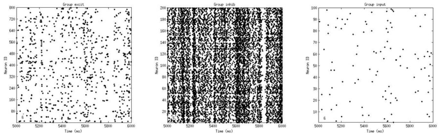
This will plot the data in bins of 1000 ms in the current figure/axes, one group per subplot, using a default plot type, which is determined by the Grid3D dimensions of each group (see 9.2.4 NetworkMonitor Plot Types and 9.3.4 GroupMonitor Plot Types). An example is shown in the figure below.
A list of frames to be plotted as well as the histogram bin window (ms) can be specified directly. For example, the following command would bin the data into frames 500 ms length, and display the first, second, and eighth frame using default plot types for each group:
The default plot type for each group can be changed via setGroupPlotType:
Plot types are managed by the GroupMonitor object. For a list of available plot types, please refer to 9.2.4 NetworkMonitor Plot Types.
Every Monitor comes with an InteractiveMode for plotting activity and weights. By default, plotting will occur at a predefined speed (5 frames per second), unless otherwise specified using the method setPlottingAttributes (see 9.2.5 NetworkMonitor Plotting Attributes). At any time, the user can hit key 'p' to pause plotting, or 'q' to quit. Hitting key 's' will enter stepping mode, which will freeze the current frame until the user either hits the 'right arrow' key (in order to step one frame forward) or the 'left arrow' key (in order to step one frame backward).
A number of additional plotting attributes can be set via setPlottingAttributes, such as the background color of the figure and the number of frames to be displayed per second (see 9.2.5 NetworkMonitor Plotting Attributes).
Certain plot types, such as 'heatmap' or 'flowfield' depend on appropriate Grid3D dimensions (2D for the former, 3D for the latter). For example, the heatmap of a population with 100 neurons on a 100x1x1 grid will be a single row. But, the grid dimensions can be reshaped on-the-fly, to make them easier to visualize:
Note that the overall number of neurons must not change when specifying new grid dimensions.
Sometimes it is useful to manually assign subplots to each group, especially for groups whose 2D grid representations are relatively wide or tall (e.g., 5x100 neurons). In this case, setGroupSubPlots can be used to make a group plot span across multiple subplots:
By default, each group gets assigned just one subplot. Make sure that each subplot is occupied by at most one group, otherwise the plot method will break.
The raw data of a spike file can also be read directly using a SpikeReader (see 9.5.2 Spike Reader).
NetworkMonitor follows the plot types that are specified and managed by GroupMonitor. For a complete list of available plot types, please refer to 9.3.4 GroupMonitor Plot Types.
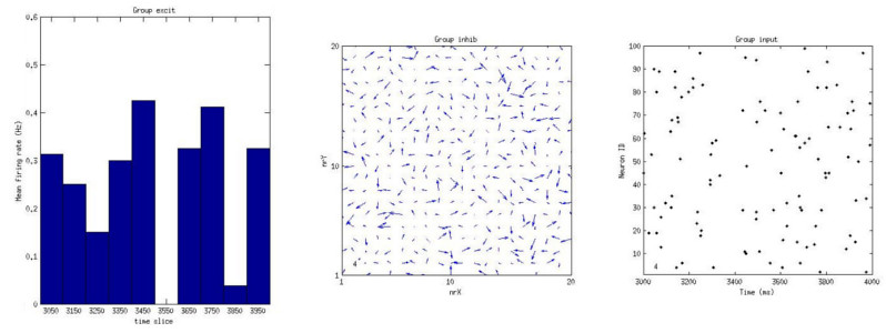
Plot types can be mixed-and-matched within a NetworkMonitor plot. For example, a network containing three groups "excit", "inhib", and "input" might be visualized with three different types:
The result of this code snippet is shown in the figure below.
setGrid3D). The method setPlottingAttributes(varargin) can be used to set default plotting attributes. These default settings will apply to all activity plots, unless their values are overwritten explicitly in the plot method (see 9.2.3 Plotting Activity).
The following command sets the value of variable propertyName1 to value value1:
Additional variables can be flexibly appended; order or capitalization does not matter. A list of available attributes can be displayed via:
Activity plots can be directly saved to AVI movie files via the following command:
This will generate a default NetworkMonitor plot (see 9.2.3 Plotting Activity) and save the frames to an .avi binary using the MATLAB VideoWriter utility.
The following command will generate file called myMovie.avi that shows group activity with default plot types, binning window 500 ms, and display the first, second, and eighth frame at a playback rate of 1 fps:
Plot types for each group can be set via setGroupPlotType (see 9.2.4 NetworkMonitor Plot Types).
setGrid3D). The method setRecordingAttributes(varargin) can be used to set default recording attributes. These default settings will apply to all recordings, unless their values are overwritten explicitly in the recordMovie method (see 9.3.6 Recording a Movie).
The following command sets the value of variable propertyName1 to value value1:
Additional variables can be flexibly appended; order or capitalization does not matter. A list of available attributes can be displayed via:
A GroupMonitor can be used to monitor properties as well as the activity of a specific neuronal group in a network. The monitor will assume that a corresponding spike file was created via SpikeMonitor during the CARLsim simulation.
The following methods are available:
The following public members (properties) are available:
In order to open a GroupMonitor, specify the name of the group (given during a CARLsim simulation via CARLsim::createGroup or CARLsim::createSpikeGeneratorGroup) and the directory in which the spike file resides (results/ by default):
By default, this will look for a spike file named spk_{group name}.dat in the results/ directory, which is the default name pattern for spike files created with CARLsim::setSpikeMonitor.
In case the spike file does not follow the default pattern, creating a GroupMonitor will result in the following warning:
and trying to call the plot method will result in an error message:
In this case, the method setSpikeFileAttributes can be used to change the default prefix and suffix of the spike file name. In the above case, the prefix would be spk_ and the suffix would be .dat. Analogously, for a spike file following the naming convention spike_{group name}.ext the prefix would be spike_ and the suffix would be .ext. After prefix/suffix have been set accordingly, the spike file will be found and activity can be plotted:
Once a GroupMonitor has been set up, activity can be plotted using the plot method:
This will plot the data in bins of 1000 ms in the current figure/axes using a default plot type, which is determined by the Grid3D dimensions of the group (see 9.3.4 GroupMonitor Plot Types).
A list of frames to be plotted as well as the histogram bin window (ms) can be specified directly. For example, the following command would bin the data into frames 500 ms length, and display the first, second, and eighth frame as a heat map:
Every Monitor comes with an InteractiveMode for plotting activity and weights. By default, plotting will occur at a predefined speed (5 frames per second), unless otherwise specified using the method setPlottingAttributes (see 9.3.5 GroupMonitor Plotting Attributes). At any time, the user can hit key 'p' to pause plotting, or 'q' to quit. Hitting key 's' will enter stepping mode, which will freeze the current frame until the user either hits the 'right arrow' key (in order to step one frame forward) or the 'left arrow' key (in order to step one frame backward).
It is also possible to set the default plot type directly, so it does not have to be specified each time data is plotted or recorded:
For a list of available plot types, please refer to 9.3.4 GroupMonitor Plot Types.
A number of additional plotting attributes can be set via setPlottingAttributes, such as the background color of the figure and the number of frames to be displayed per second (see 9.3.5 GroupMonitor Plotting Attributes).
Certain plot types, such as 'heatmap' or 'flowfield' depend on appropriate Grid3D dimensions (2D for the former, 3D for the latter). For example, the heatmap of a population with 100 neurons on a 100x1x1 grid will be a single row. But, the grid dimensions can be reshaped on-the-fly, to make them easier to visualize:
Note that the overall number of neurons must not change when specifying new grid dimensions.
The raw data of a spike file can also be read directly using a SpikeReader (see 9.5.2 Spike Reader).
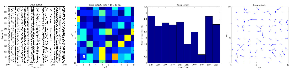
The following image illustrates the different plot types that are available (applied to an arbitrary network):
A specific default plot type can be set using setDefaultPlotType:
where str is either 'flowfield', 'heatmap', 'histogram', or 'raster'. This type will then apply to all subsequent plotting and recording commands, unless it is overwritten explicitly with one of the method's input arguments.
This value can be overwritten by explicitly specifying a plot type when using the methods plot (see 9.3.3 Plotting Activity) or recordMovie (see 9.3.6 Recording a Movie).
Plot type 'flowfield' will plot a 2D vector field where the length of the vector is given as the firing rsate of the neuron times the corresponding vector orientation. The latter is inferred from the third Grid3D dimension, z. For example, Grid3D(10,10,4) plots a 10x10 vector flow field, assuming that neurons with z=0 code for direction=0deg, z=1 corresponds to direction=90deg, z=2 is 180deg, and z=3 is 270deg. Vectors with length smaller than 10% of the max in each frame are not shown.
Plot type 'heatmap' will plot a topographical map of group activity (based on Grid3D) where hotter colors mean higher firing rate.
Plot type 'histogram' will plot a histogram of firing rates in the group. The number of bins and whether to plot firing rates (Hz) instead of number of spikes can be set with options 'histNumBins' and 'histShowRate' in method setPlottingAttributes.
Plot type 'raster' will output the data as a raster plot with bin window binWindowMs.
setGrid3D). The method setPlottingAttributes(varargin) can be used to set default plotting attributes. These default settings will apply to all activity plots, unless their values are overwritten explicitly in the plot method (see 9.3.3 Plotting Activity).
The following command sets the value of variable propertyName1 to value value1:
Additional variables can be flexibly appended; order or capitalization does not matter. A list of available attributes can be displayed via:
Activity plots can be directly saved to AVI movie files via the following command:
This will generate a default GroupMonitor plot (see 9.3.3 Plotting Activity) and save the frames to an .avi binary using the MATLAB VideoWriter utility.
The following command will generate file called myMovie.avi that shows a heat map of group activity with binning window 500 ms, and display the first, second, and eighth frame at a playback rate of 1 fps:
setGrid3D). The method setRecordingAttributes(varargin) can be used to set default recording attributes. These default settings will apply to all recordings, unless their values are overwritten explicitly in the recordMovie method (see 9.3.6 Recording a Movie).
The following command sets the value of variable propertyName1 to value value1:
Additional variables can be flexibly appended; order or capitalization does not matter. A list of available attributes can be displayed via:
A ConnectionMonitor can be used to monitor properties as well as the synaptic weights of a specific connection in a network (specified via CARLsim::connect). The monitor will assume that a corresponding weight file was created via ConnectionMonitor during the CARLsim simulation.
The following methods are available:
The following public members (properties) are available:
In order to open a ConnectionMonitor, specify the name of the pre-synaptic and post-synaptic group (given during a CARLsim simulation via CARLsim::createGroup or CARLsim::createSpikeGeneratorGroup) and the directory in which the connect file resides (results/ by default):
By default, this will look for a connect file named conn_{pre-group name}_{post-group name}.dat in the results/ directory, which is the default name pattern for connect files created with CARLsim::setConnectionMonitor.
In case the connect file does not follow the default pattern, creating a ConnectionMonitor will result in the following warning:
and trying to call the plot method will result in an error message:
In this case, the method setConnectFileAttributes can be used to change the default prefix, suffix, and separator of the connect file name. In the above case, the prefix would be conn_, the separator would be _, and the suffix would be .dat. Note that only the "_" between group names counts as the separator. Analogously, for a connect file following the naming convention connect_{pre-group name}-{post-group name}.ext the prefix would be connect_, the separator would be -, and the suffix would be .ext. After prefix/suffix/separator have been set accordingly, the connect file will be found and weights can be plotted:
Once a ConnectionMonitor has been set up, synaptic weights can be plotted using the plot method:
This will plot each weight snapshot (or frame) in the current figure/axes using a default plot type, which is determined by the size of the weight matrix (see 9.4.4 ConnectionMonitor Plot Types).
A list of frames (or snapshots) and neurons to be plotted can be specified directly. For example, the following command would display the first, second, and eighth weight snapshot as a 2D heat map:
Every Monitor comes with an InteractiveMode for plotting activity and weights. By default, plotting will occur at a predefined speed (5 frames per second), unless otherwise specified using the method setPlottingAttributes (see 9.4.5 ConnectionMonitor Plotting Attributes). At any time, the user can hit key 'p' to pause plotting, or 'q' to quit. Hitting key 's' will enter stepping mode, which will freeze the current frame until the user either hits the 'right arrow' key (in order to step one frame forward) or the 'left arrow' key (in order to step one frame backward).
It is also possible to set the default plot type directly, so it does not have to be specified each time data is plotted or recorded:
For a list of available plot types, please refer to 9.4.4 ConnectionMonitor Plot Types.
A number of additional plotting attributes can be set via setPlottingAttributes, such as the background color of the figure and the number of frames to be displayed per second (see 9.4.5 ConnectionMonitor Plotting Attributes).
It is also possible to display weight data only for a subset of pre-synaptic or post-synaptic neurons. This makes it possible to visualize the receptive field of a post-synaptic neuron, or the response field of a pre-synaptic neuron.
The raw data of a connect file can also be read directly using a ConnectionReader (see 9.5.3 Connection Reader).
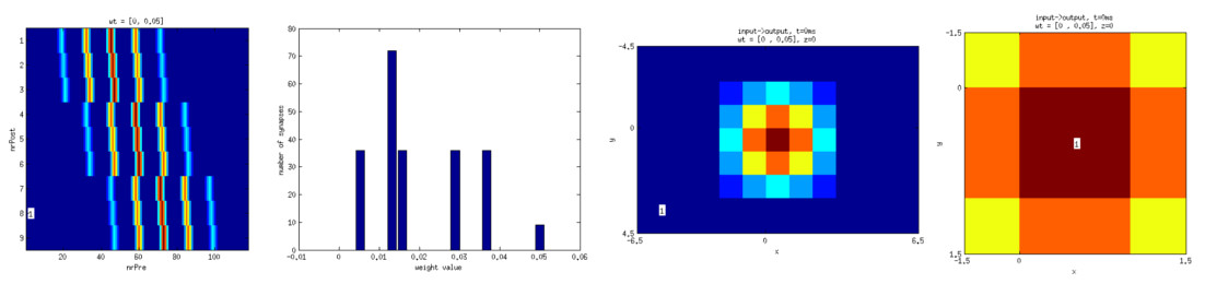
The following image illustrates the different plot types that are available (applied to the small "Hello World" network, which consists of 13x9 neurons projecting to 3x3 neurons with Gaussian connectivity):
A specific default plot type can be set using setDefaultPlotType:
where str is either 'heatmap', 'histogram', 'receptivefield', or 'responsefield'. This type will then apply to all subsequent plotting and recording commands, unless it is overwritten explicitly with one of the method's input arguments.
This value can be overwritten by explicitly specifying a plot type when using the methods plot (see 9.4.3 Plotting Weights) or recordMovie (see 9.4.6 Recording a Movie).
Plot type 'heatmap' will plot a 2D weight matrix where the first dimension corresponds to the number of neurons in the pre-synaptic group (labeled nrPre in the image above), and the second dimension corresponds to the number of neurons in the post-synaptic group (labeled nrPost in the image above).
Plot type 'histogram' will plot a histogram of all weight values in the connection.
Plot type 'receptivefield' will plot the spatial receptive field of post-synaptic neurons (looking back on all connected pre-synaptic neurons). By default, the receptive field of all neurons will be shown. An additional argument to plot allows to specify a list of neurons for which to show the receptive field. For example, the receptive field in the above image (third panel) was generated with:
shown for the first frame and the fifth neuron in the post-synaptic group (which is located at (0,0,0)).
Plot type 'responsefield' will plot the spatial response field of pre-synaptic neurons (looking forward on all connected post-synaptic neurons). By default, the response field of all neurons will be shown. An additional argument to plot allows to specify a list of neurons for which to show the response field. For example, the response field in the above image (fourth panel) was generated with:
shown for the first frame and the 59th neuron in the pre-synaptic group (which is located at (0,0,0)).
The method setPlottingAttributes(varargin) can be used to set default plotting attributes. These default settings will apply to all activity plots, unless their values are overwritten explicitly in the plot method (see 9.4.3 Plotting Weights).
The following command sets the value of variable propertyName1 to value value1:
Additional variables can be flexibly appended; order or capitalization does not matter. A list of available attributes can be displayed via:
Activity plots can be directly saved to AVI movie files via the following command:
This will generate a default ConnectionMonitor plot (see 9.4.3 Plotting Weights) and save the frames to an .avi binary using the MATLAB VideoWriter utility.
The following command will generate file called myMovie.avi that shows a heat map of the weight matrix, and display the first, second, and eighth frame (or snapshot) at a playback rate of 1 fps:
The method setRecordingAttributes(varargin) can be used to set default recording attributes. These default settings will apply to all recordings, unless their values are overwritten explicitly in the recordMovie method (see 9.4.6 Recording a Movie).
The following command sets the value of variable propertyName1 to value value1:
Additional variables can be flexibly appended; order or capitalization does not matter. A list of available attributes can be displayed via:
Although the OAT provides a variety of functions to simplify the visualization and analysis of network activity or topology, there might be cases in which the user might like to have complete control over the process. Therefore, CARLsim also provides a means to directly read the simulation, spike, and weight file binaries generated during a simulation.
A SimulationReader can be used to read a simulation log file that is created by default by every CARLsim simulation, or by explicitly calling CARLsim::saveSimulation. This allows to directly access important properties of the simulation run or the spiking network, without the need of a NetworkMonitor.
The following public members (properties) are available:
The following code snippet points a SimulationReader to a simulation file results/sim_myNet.dat and populates the public member structs sim and groups with viable simulation/network information:
The sim struct can then be queried for values such as simulation time or execution time:
The groups struct can then be queried for values such as the Grid3D dimensions or neuron IDs:
By default, the deprecated syn_* properties will not be populated by the constructor call. In order to access these properties, the constructor needs to be called with an additional flag loadSynapseInfo:
Note that for this to work, the simulation must have been saved with CARLsim::saveSimulation input argument saveSynapseInfo set to true.
syn_* properties above is deprecated. Use ConnectionMonitor or ConnectionReader to access synapse information instead. A SpikeReader can be used to read raw spike file data that was generated with the SpikeMonitor utility in CARLsim. This allows to directly access the spike data, be it in AER format or binned in suitable time windows, without the need of a GroupMonitor or NetworkMonitor.
The following methods are available:
The following public members (properties) are available:
The following code snippet points a SpikeReader object to a spike file results/spk_group1.dat (generated with the SpikeMonitor utility in CARLsim) and returns the spike data binned into 100 ms time windows:
The variable spkData will return spike data in a 2D matrix, where the first dimension corresponds to the bin windows and the second dimension corresponds to the number of neurons in the group (1-indexed). For example, with a binning window of 100ms, spkData(1,1) would contain the number of spikes that the first neuron in the group emitted in the first 100ms (t = 0 .. 99ms) of the simulation.
Alternatively, spike data can be returned in AER format (as [times;neurIds]) if the binWindowMs input argument to readSpikes is set to -1:
The generation of a raster plot is then as easy as:
The SpikeReader can also be queried for an estimate about the total simulation duration via:
Note that this is only an estimate, based on the last spike time in the group. Other than that, a SpikeReader object does not know about any simulation procedures.
A ConnectionReader can be used to read raw connection file data that was generated with the ConnectionMonitor utility in CARLsim. This allows to directly access the weight data, at specific times, without the need of a ConnectionMonitor.
The following methods are available:
The following public members (properties) are available:
The following code snippet points a ConnectionReader object to a connection file results/conn_group1_group2.dat (generated with the ConnectionMonitor utility in CARLsim) and returns the weight data for all recorded snapshots:
The variable allTimestamps will contain a list of timestamps (ms) at which the corresponding weights were recorded. The variable allWeights will return the weight data in a 2D matrix, where the first dimension specifies the snapshot number and the second dimension corresponds to all synaptic weights for that specific snapshot. For example, allWeights(1,:) would contain all synaptic weights recorded during the first snapshot. The timestamp of the first snapshot can be retrieved via allTimestamps(1).
Plotting a histogram of all weights is then as easy as:
Alternatively, the weight vector can be reshaped as a 2D weight matrix according to the population dimensions and plotted as a heatmap:
Please note that the following scripts from CARLsim 2.2 (from former directory scripts/common/) are no longer available:
readFramesFromRgbFile.m: replaced with VisualStimulus Toolbox (see 6.3 Visual Stimulus Toolbox)readNetwork.m: replaced with NetworkMonitors (see 9.2 NetworkMonitor)readSpikes.m: replaced with Spike Readers (see 9.5.2 Spike Reader)readSpikesAERtoFull.m: no longer availablewriteFramesToRgbFile.m: replaced with VisualStimulus Toolbox (see 6.3 Visual Stimulus Toolbox)  1.8.11
