In this tutorial we will implement an 80-20 random spiking neural network with synapses of varying axonal delay that are subject to spike-timing dependent plasticity (STDP). We follow the MATLAB implementation spnet.m, which can be obtained from Izhikevich's Website. In addition, we will use various functions from the MATLAB Offline Analysis Toolbox (OAT) to visualize network activity and weight changes.

At the end of the tutorial, you will know how to:

set up a 80-20 network of Izhikevich spiking neurons
inject current into the network
set up E-STDP and I-STDP for specific groups
run a network in CUBA mode
use a NetworkMonitor to visualize network activity (OAT)
use a ConnectionMonitor to visualize weight changes (OAT)

This tutorial assumes you know how to:

run a simple CARLsim program (see Tutorial 1: Basic Concepts)

The source code of this tutorial can be found in %%CARLSIM_ROOT_DIR%%/doc/source/tutorial/2_random_spnet.

2.1 80-20 Networks

80-20 networks get their name from the ratio of excitatory (80%) to inhibitory (20%) neurons in the network, which is thought to preserve a ratio found in the mammalian cortex (Braitenberg & Schuz, 1991), although these numbers might not be exact.

Such networks are supposed to exhibit sleeplike oscillations, gamma (40 Hz) rhythms, conversion of firing rates to spike timings, and other interesting regimes.

2.2 Network Setup

As always, the first step in setting up a CARLsim program is to include the libCARLsim library and to instantiate the main simulation object:

#include <carlsim.h>
#include <vector>
int main(int argc, const char* argv[]) {
    CARLsim sim("spnet", GPU_MODE, USER);

2.2.1 CONFIG State

From then on, the simulation is in CONFIG_STATE, allowing the properties of the neural network to be specified. In this tutorial, we consider a network of 800 excitatory (regular spiking; RS) and 200 inhibitory neurons (fast spiking; FS) (see 3.1.1 Izhikevich Neurons (4-Parameter Model)). Each neuron shall have roughly 100 incoming synapses (nSynPerNeur) with axonal delays between 1ms and 20ms (maxDelay). We first set a number of parameters:

int nNeur = 1000;           // number of neurons
int nNeurExc = 0.8*nNeur;   // number of excitatory neurons
int nNeurInh = 0.2*nNeur;   // number of inhibitory neurons
int nSynPerNeur = 100;      // number of synpases per neuron
int maxDelay = 20;          // maximal conduction delay

and then create the groups of regular spiking and fast spiking neurons with appropriate Izhikevich parameters a, b, c, and d:

// create 80-20 network with 80% RS and 20% FS neurons
int gExc = sim.createGroup("exc", nNeurExc, EXCITATORY_NEURON);
sim.setNeuronParameters(gExc, 0.02f, 0.2f, -65.0f, 8.0f); // RS
int gInh = sim.createGroup("inh", nNeurInh, INHIBITORY_NEURON);
sim.setNeuronParameters(gInh, 0.1f, 0.2f, -65.0f, 2.0f); // FS

The network considered here is sparse with 10% probability of connection between any two neurons (the probability is found by dividing the number of synpases per neuron by the number of neurons):

float pConn = nSynPerNeur*1.0f/nNeur; // connection probability

We also set the synaptic weight magnitudes to be 6.0f for excitatory synapses and 5.0f for inhibitory synapses, and make sure weight magnitudes never get larger than 10.0f:

// specify connectivity
float wtExc = 6.0f;                   // synaptic weight magnitude if pre is exc
float wtInh = 5.0f;                   // synaptic weight magnitude if pre is inh (no negative sign)
float wtMax = 10.0f;                  // maximum synaptic weight magnitude

Then the synaptic connections can be specified. Groups are connected with the "random" primitive type of CARLsim::connect that sparsely connects groups with a fixed connection probability. Weights are initialized to wtExc and wtInh for excitatory and inhibitory synapses, respectively. Note that the weight of inhibitory synapses in RangeWeight is to be understood as a weight magnitude, and therefore does not have a negative sign. Weights are bounded by the interval [0, wtMax]. Axonal delays are uniformly distributed in the range [1, 20] ms. Connections should not be further confined to a spatial receptive field, which is denoted by RadiusRF(-1). SYN_PLASTIC denotes that the synapses will be subject to plasticity. All of this is accomplished with the following code snippet:

// gExc receives input from nSynPerNeur neurons from both gExc and gInh
// every neuron in gExc should receive ~nSynPerNeur synapses
sim.connect(gExc, gExc, "random", RangeWeight(0.0f, wtExc, wtMax), pConn, RangeDelay(1,20), RadiusRF(-1), SYN_PLASTIC);
sim.connect(gInh, gExc, "random", RangeWeight(0.0f, wtInh, wtMax), pConn, RangeDelay(1,20), RadiusRF(-1), SYN_PLASTIC);
// gInh receives input from nSynPerNeur neurons from gExc, all delays are 1ms, no plasticity
// every neuron in gInh should receive ~nSynPerNeur synapses
sim.connect(gExc, gInh, "random", RangeWeight(wtExc), pConn*nNeur/nNeurExc);

What remains to be done is to enable STDP on the connections above. STDP is enabled post-synaptically: Setting E-STDP will enable STDP on all incoming excitatory synapses (where the pre-synaptic group is excitatory), whereas setting I-STDP will enable STDP on all incoming inhibitory synapses (where the pre-synaptic group is inhibitory). We enable both types on post-synaptic group gExc (but not gInh on to be consistent with the original MATLAB code) and set the shape of the STDP curve to the standard exponential curve (see 5.2.2 Excitatory STDP (E-STDP) and Inhibitory STDP (I-STDP)):

// enable STDP on all incoming synapses to gExc
float alphaPlus = 0.1f, tauPlus = 20.0f, alphaMinus = 0.1f, tauMinus = 20.0f;
sim.setESTDP(gExc, true, STANDARD, ExpCurve(alphaPlus, tauPlus, -alphaMinus, tauMinus));
sim.setISTDP(gExc, true, STANDARD, ExpCurve(-alphaPlus, tauPlus, alphaMinus, tauMinus));

Note the sign of the alpha variables. "Standard" E-STDP implies positive weight changes for pre-before-post events (alphaPlus) and negative weight changes for post-before-pre (-alphaMinus). With I-STDP the logic is inverted.

Finally, we disable synaptic conductances so that the network is run in CUBA mode (see 3.2.1 CUBA):

// run CUBA mode

sim.setConductances(false);

2.2.2 SETUP State

Once the spiking network has been specified, the function CARLsim::setupNetwork optimizes the network state for the chosen back-end (CPU or GPU) and moves the simulation into SETUP_STATE:

// ---------------- SETUP STATE -------------------

sim.setupNetwork();

In this state, we specify a number of SpikeMonitor and ConnectionMonitor objects to record network activity and synaptic weights to a "DEFAULT" binary file (see Chapter 7: Monitoring):

SpikeMonitor* SMexc = sim.setSpikeMonitor(gExc, "DEFAULT");
SpikeMonitor* SMinh = sim.setSpikeMonitor(gInh, "DEFAULT");
sim.setConnectionMonitor(gExc, gExc, "DEFAULT");
sim.setConnectionMonitor(gInh, gExc, "DEFAULT");

This will dump all spikes of group gExc (in AER format) to a binary with default file name "results/spk_exc.dat", where "exc" is the name that was assigned to the group gExc in the call to CARLsim::createGroup above. The same is true for group gInh. Analogously, two weight files "results/conn_exc_exc.dat" and "results/conn_inh_exc.dat" will be created that contain snapshots of the synaptic weights taken every 10,000ms.

2.2.3 RUN State

The first call to CARLsim::runNetwork will take the simulation into RUN_STATE. The simulation will be repeatedly run (or "stepped") for 1ms, up to the point at which a total of 10,000ms are simulated.

The main simulation loop is encapsulated by a pair of SpikeMonitor::startRecording and SpikeMonitor::stopRecording calls, which instruct the SpikeMonitor objects to keep track of all spikes emitted by the neurons in their monitored group (see 7.1.2.1 Start and Stop Recording):

// ---------------- RUN STATE -------------------
SMexc->startRecording();
SMinh->startRecording();
for (int t=0; t<10000; t++) {
    // main simulation loop
    // etc.
}
SMexc->stopRecording();
SMinh->stopRecording();

After (or during) the simulation these objects could be queried for more detailed spike metrics (see 7.1.2.3 Spike Metrics), but for the sake of simplicity we will only print a condensed version of spike statistics at the end:

// print firing stats (but not the exact spike times)
SMexc->print(false);
SMinh->print(false);

Finally, the main simulation loop consists of repeatedly stepping the model for 1ms. At every step we randomly choose a single neuron in the network to receive an external (thalamic) input current of 20.0f. To achieve this, we maintain a vector of external currents for every neuron in the group, initialized to zero:

// random thalamic input to a single neuron from either gExc or gInh
std::vector<float> thalamCurrExc(nNeurExc, 0.0f);
std::vector<float> thalamCurrInh(nNeurInh, 0.0f);

Then, a neuron ID is chosen randomly, and the corresponding input current for the identified neuron is adjusted:

int randNeurId = round( drand48()*(nNeur-1) );
float thCurr = 20.0f;
if (randNeurId < nNeurExc) {
    // neurId belongs to gExc
    thalamCurrExc[randNeurId] = thCurr;
} else {
    // neurId belongs to gInh
    thalamCurrInh[randNeurId - nNeurExc] = thCurr;
}

Finally, the resulting vectors are applied to both groups. Note that we explicitly set the unaffected input currents to zero every time step. This is because otherwise the non-zero input current from previous iterations will keep getting applied until manually reset to zero:

sim.setExternalCurrent(gExc, thalamCurrExc);

sim.setExternalCurrent(gInh, thalamCurrInh);

After that is accomplished, the model is stepped for 1ms while explicitly disabling printing the run summary at the end:

// run for 1 ms, don't generate run stats

sim.runNetwork(0,1,false);

2.3. Network Output

After navigating to %CARLSIM_ROOT_DIR%%/doc/source/tutorial/2_random_spnet, the network can be compiled and run with the following commands (on Unix):

$ make

$ ./random_spnet

On Windows, the .vcxproj file is already added to the CARLsim.sln solution file. Thus the project can be built simply by opening the solution file in Visual Studio, by right-clicking the project directory and choosing "Build project".

Some of the CARLsim output is shown below:

****************      Initializing GPU Simulation      *************************
GPU Memory Management: (Total 2.999 GB)
Data          Size        Total Used  Total Available
Init:         2.999 GB    0.221 GB    2.779 GB
Ntw Params:   0.000 GB    0.221 GB    2.779 GB
Static Load:  0.001 GB    0.222 GB    2.778 GB
Group Id:     0.000 GB    0.222 GB    2.778 GB
Conn Info:    0.004 GB    0.226 GB    2.774 GB
State Info:   0.004 GB    0.229 GB    2.770 GB
SpikeMonitor set for group 0 (exc)
SpikeMonitor set for group 1 (inh)
ConnectionMonitor 0 set for Connection 0: 0(exc) => 0(exc)
ConnectionMonitor 1 set for Connection 1: 1(inh) => 0(exc)
(t=10.000s) SpikeMonitor for group exc(0) has 31890 spikes in 10000 ms (3.99 +/- 0.97 Hz)
(t=10.000s) SpikeMonitor for group inh(1) has 46688 spikes in 10000 ms (23.34 +/- 3.00 Hz)
*******************      GPU Simulation Summary      ***************************
Network Parameters:   numNeurons = 1000 (numNExcReg:numNInhReg = 80.0:20.0)
                      numSynapses = 100436
                      maxDelay = 20
Simulation Mode:      CUBA
Random Seed:          1425923871
Timing:               Model Simulation Time = 10 sec
                      Actual Execution Time = 2.92 sec
Average Firing Rate:  2+ms delay = 9.961 Hz
                      1ms delay = 0.000 Hz
                      Overall = 7.968 Hz
Overall Firing Count: 2+ms delay = 79685
                      1ms delay = 0
                      Total = 79685
********************************************************************************

Since the network was run in GPU_MODE, the simulation will print a summary of the GPU memory management. This indicates the amount of GPU memory that each important data structure occupies. The above was generated on a GTX 780 with 3GB of GPU memory.

Both SpikeMonitor objects produced one line of output each at the end of the simulation via SpikeMonitor::print. This line includes the number of spikes each group emitted over the time course of 10,000ms, with corresponding mean firing rate (in Hz) and standard deviation given in parentheses.

At the end of the simulation, a summary is printed that confirms the 80-20 ratio of excitatory to inhibitory neurons. A total number of 100,436 synapses were created, confirming the attempted number of (roughly) 100 synapses per neuron. The network was simulated for 10 seconds, yet its execution took only 2.92 seconds of wall-clock time, which means the network was run 3.42 times faster than real-time.

2.4. Visualizing Network Activity and Weight Changes

In order to plot network activity and observe weight changes in the network, we will make use of the MATLAB Offline Analysis Toolbox (OAT) (see Chapter 9: MATLAB Offline Analysis Toolbox (OAT)).

The Tutorial subdirectory "scripts/" provides a MATLAB script "scripts/demoOAT.m" to demonstrate the usage of the OAT. The script looks like this:

% OAT demo
% first, init OAT by adding path
initOAT
% second, open a NetworkMonitor on the simulation file
% and plot the activity of the network
NM = NetworkMonitor('../results/sim_spnet.dat')
NM.plot
% third, observe weight changes in the network
CM0 = ConnectionMonitor('exc','exc','../results')
CM0.plot('histogram')
CM1 = ConnectionMonitor('inh','exc','../results')
CM1.plot('histogram')

After adding the location of the OAT source code to the MATLAB path, a NetworkMonitor is opened on the simulation file "../results/sim_spnet.dat", which was automatically created during the CARLsim simulation (note that the string "spnet" corresponds to the name given to the network in the CARLsim constructor).

Calling the plot method will then visualize network activity using default settings and a plot type that depends on the spatial structure of the neuron groups. Since the network does not have any particular spatial structure, the default plot type is a raster plot, shown in frames of 1000ms, as seen in Fig. 1 below.

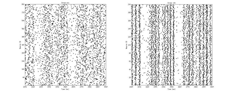
Fig. 1. NetworkMonitor output for groups 'exc' and 'inh' (raster plot)

Fig. 2 shows the temporal evolution of weights from the recurrent excitatory connection on gExc. At the beginning of the experiment (leftmost panel), all weights are initialized to 6.0f. Over time, these values start to diverge, but stay confined in the range [0.0f, 10.0f].

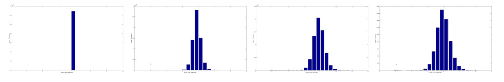
Fig. 2. ConnectionMonitor output for the connection 'exc'=>'exc' (histogram)

Similar behavior can be observed on the connection from gInh to gExc.

It would also be possible to open a ConnectionMonitor on the fixed connection from gExc to gInh, but the expected output would be similar to the leftmost panel of Fig. 2, showing all weights initialized to 5.0f, with no weight changes to report over time.

Table of Contents