In this tutorial, we will take a closer look at CARLsim's spatial connectivity profiles by implementing a simple image filter. Specifically, we will use the Gaussian connectivity profile to implement a smoothening operation and an edge detector (using a difference of Gaussians). To make this work, we will make use of both the Offline Analysis Toolbox and the Visual Stimulus Toolbox.

At the end of the tutorial, you will know how to:

implement Gaussian connectivity profiles
use the Grid3D and RadiusRF structs for 2-D and 3-D transforms
import stimuli from the VisualStimulusToolbox into CARLsim
set up a custom SpikeGenerator object
create Gaussian connections for neurons arranged on a 2D/3D grid

The source code of this tutorial can be found in %%CARLSIM_ROOT_DIR%%/doc/source/tutorial/4_image_processing.

4.1 VisualStimulusToolbox

CARLsim uses VisualStimulusToolbox in MATLAB to convert images into binary files that CARLsim can understand.

VisualStimulusToolbox is a lightweight MATLAB toolbox for generating, storing, and plotting 2D visual stimuli commonly used in vision and neuroscience research, such as sinusoidal gratings, plaids, random dot fields, and noise. Every stimulus can be plotted, recorded to AVI, and stored to binary:

4.1.1 Installing VisualStimulusToolbox

VisualStimulusToolbox is available on GitHub, but CARLsim comes pre-installed with an appropriate version of it (see external/VisualStimulusToolbox).

If you followed the CARLsim installation instructions outlined in Chapter 1: Getting Started, you are already good to go!

However, if your external/VisualStimulusToolbox directory is empty (e.g., because you forgot the –recursive flag when you cloned CARLsim), you have to initialize the submodule yourself. Simply navigate to the CARLsim root directory and run the following:

$ git submodule update --init --recursive

The scripts below will automatically add the toolbox to your MATLAB path. Alternatively, you can install the toolbox as an add-on (MATLAB R2016a and newer): To open the Add-On Manager, go to the Home tab, and select Add-Ons > Manage Add-Ons.

See also: http://uci-carl.github.io/VisualStimulusToolbox

4.1.2 First Steps

To make sure VisualStimulusToolbox has been installed correctly, try opening an image file. In MATLAB, navigate to the input directory of this tutorial, then type:

>> pic = PictureStim('carl.jpg')
pic = 
  PictureStim with properties:
                  width: 2182
                 height: 2255
               channels: 1
                 length: 1
                   stim: [2255x2182 double]
    supportedNoiseTypes: {'gaussian'  'localvar'  'poisson'  'salt & pepper'  'speckle'}

You can then have a look at the picture you just loaded by typing:

>> pic.plot()

CARL logo

4.1.3 Converting an Image

In order to convert an image, you can use the script createStimFromImage.m located in the scripts folder of this tutorial.

The script is executed as follows:

>> createStimFromImage('../input/carl.jpg', '../input/carl.dat', [256 256], 'gray')

This will resize the grayscale image ../input/carl.jpg to 256x256 pixels and store the image in a binary format that CARLsim can understand (../input/carl.dat).

4.2 Gaussian Blur

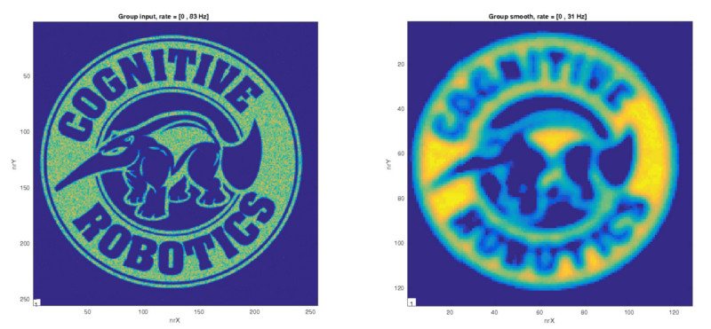
The first image processing technique we will look at is Gaussian smoothening. This technique is implemented in main_smooth.cpp.

4.2.1 Importing the Image

The idea is to assign every pixel in the image to a neuron in the spiking network. In order to preserve spatial relationships, we arrange all neurons in a grid that matches the image dimensions. The image is simply imported by:

VisualStimulus stim("input/carl.dat");

4.2.2 Assigning Image Pixels to Neurons

We can create a Grid3D struct from the stim dimensions:

Grid3D imgDim(stim.getWidth(), stim.getHeight(), stim.getChannels());

We also want a grid for the downscaled, blurred version of the image:

Grid3D imgSmallDim(imgDim.width/2, imgDim.height/2, 1);

So all we need to do is create groups with the above grids:

// ---------------- CONFIG STATE -------------------
CARLsim sim("smooth", GPU_MODE, USER);
int gIn = sim.createSpikeGeneratorGroup("input", imgDim, EXCITATORY_NEURON);
int gSmooth = sim.createGroup("smooth", imgSmallDim, EXCITATORY_NEURON);
sim.setNeuronParameters(gSmooth, 0.02f, 0.2f, -65.0f, 8.0f);

4.2.3 Performing the Smoothing

The Gaussian blur is simply implemented by a Gaussian connection. The trick is to use the RadiusRF struct to define the Gaussian kernel. For image processing, we want a Gaussian kernel in x and y dimensions, such as a 5x5 kernel. This is equivalent to RadiusRF(5, 5, 0). Here, the zero specifies that the smoothing will be performed separately for every channel (third dimension). If we wanted to smooth over the third dimension (e.g., a Gaussian voxel), we would choose RadiusRF(5, 5, 5).

However, what we really want is to sum or average over all three color channels if the image is RGB. We do this by specifying RadiusRF(5, 5, -1):

sim.connect(gIn, gSmooth, "gaussian", RangeWeight(2.0f), 1.0f,

RangeDelay(1), RadiusRF(5,5,-1));

We set up some SpikeMonitor objects so that we can have a look at the output:

// ---------------- SETUP STATE -------------------
sim.setupNetwork();
sim.setSpikeMonitor(gIn, "DEFAULT");
sim.setSpikeMonitor(gSmooth, "DEFAULT");

We then read the pixels of the image using the VisualStimulus bindings:

PoissonRate* rates = stim.readFramePoisson(50.0f, 0.0f);

This reads all pixel values and normalizes them in the range [0, 50Hz], such that white pixels (grayscale value 255) is assigned to 50 Hz, and 0 is 0.

The PoissonRate object that is returned from this call neatly fits into CARLsim::setSpikeRate:

sim.setSpikeRate(gIn, rates);

Then all that is left to do is run the network:

sim.runNetwork(1,0); // run the network

This works for movies as well (where the number of frames > 1). For this, we simply wrap the above commands in a for loop, and repeated calls to readFrame will simply process the next frame in the loop:

// ---------------- RUN STATE -------------------
for (int i=0; i<stim.getLength(); i++) {
    PoissonRate* rates = stim.readFramePoisson(50.0f, 0.0f);
    sim.setSpikeRate(gIn, rates);
    sim.runNetwork(1,0); // run the network
}

And done!

4.2.4 Visualizing the Output

You can compile and run the above network as follows:

$ make smooth

$ ./smooth

The result can then be analyzed using the OAT. Visualizing network activity is easiest with the NetworkMonitor. Go back to the scripts folder in MATLAB, and run:

>> demoSmooth

Gaussian smoothing using CARLsim

4.3 Difference of Gaussians: Edge Detection

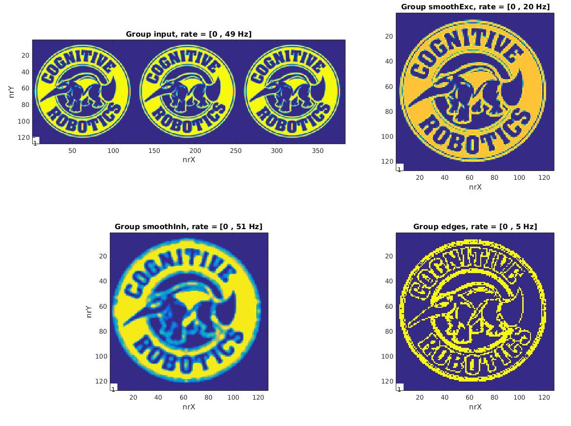
We can extend the above example by implementing an edge detector using a difference of Gaussians (DOG) operation. For this, we will first convolve the image with a small Gaussian kernel RadiusRF(0.5, 0.5, -1), which is basically a "one-to-one" connection. From the output of this operation, we will then subtract a blurred version of the image. The result will be an edge map.

4.3.1 Setting up the Network

Importing the image and setting up the Grid3D structs is the same as above:

CARLsim sim("dog", GPU_MODE, USER);
VisualStimulus stim("input/carl.dat");
stim.print();
Grid3D imgDim(stim.getWidth(), stim.getHeight(), stim.getChannels());
Grid3D imgSmallDim(imgDim.width/2, imgDim.height/2, 1);

From these specs, we will create the input and smoothing groups as above:

int gIn = sim.createSpikeGeneratorGroup("input", imgDim, EXCITATORY_NEURON);
int gSmoothExc = sim.createGroup("smoothExc", imgSmallDim, EXCITATORY_NEURON);
sim.setNeuronParameters(gSmoothExc, 0.02f, 0.2f, -65.0f, 8.0f);

However, this time around we also need an inhibitory group, so that we can subtract the blurred version of the image, and an output group that will contain the edge map:

int gSmoothInh = sim.createGroup("smoothInh", imgSmallDim, INHIBITORY_NEURON);
sim.setNeuronParameters(gSmoothInh, 0.02f, 0.2f, -65.0f, 8.0f);
int gEdges = sim.createGroup("edges", imgSmallDim, EXCITATORY_NEURON);
sim.setNeuronParameters(gEdges, 0.02f, 0.2f, -65.0f, 8.0f);

4.3.2 Performing the Difference of Gaussians (DOG) Operation

Setting up the connectivity is straightforward, too. The only annoying thing is that you will have to tune the synaptic weights in order to get this right.

Luckily I have already done this for you. We need two feedforward connections from the input group: One with a small kernel to an excitatory group, and another with a larger kernel to an inhibitory group.

sim.connect(gIn, gSmoothExc, "gaussian", RangeWeight(10.0f), 1.0f,
    RangeDelay(1), RadiusRF(0.5,0.5,-1));
sim.connect(gIn, gSmoothInh, "gaussian", RangeWeight(5.0f), 1.0f,
    RangeDelay(1), RadiusRF(3,3,-1));

We then want to subtract the output of gSmoothInh from gSmoothExc:

sim.connect(gSmoothExc, gEdges, "one-to-one", RangeWeight(16.0f), 1.0f,
    RangeDelay(1));
sim.connect(gSmoothInh, gEdges, "one-to-one", RangeWeight(100.0f), 1.0f,
    RangeDelay(1));

4.3.3 Converting Pixels to Spikes

This time around, we want the input to be a little more exact than a Poisson rate. The problem with the Poisson distribution is that the actual firing rate you get from a specified mean firing rate lambda has variance equal to lambda!

A more exact translation would be to convert the grayscale value of a pixel to a constant inter-spike interval (ISI), so that the firing rate of the corresponding neuron is 1/ISI.

We do this by subclassing SpikeGenerator and creating our own spike generator class:

class ConstantISI : public SpikeGenerator {
public:
    ConstantISI(int numNeur) {
        _numNeur = numNeur;
    }
    ~ConstantISI() {}
    ...
private:
    int _numNeur;
    std::vector<int> _isi;
};

The class has a private integer _numNeur that holds the number of neurons in the group, and a vector _isi that holds the ISI for every neuron in the group.

We then need to specify a nextSpikeTime method. This method is supposed to return the next spike time of a specific neuron nid in the group grpId. In our case, the next spike time is simply: the last spike of the neuron plus its ISI:

unsigned int nextSpikeTime(CARLsim* sim, int grpId, int nid, unsigned int currentTime,
    unsigned int lastScheduledSpikeTime, unsigned int endOfTimeSlice)
{
    // printf("_numNeur=%d, getGroupNumNeurons=%d\n",_numNeur, sim->getGroupNumNeurons(grpId));
    assert(_numNeur == sim->getGroupNumNeurons(grpId));
    // periodic spiking according to ISI
    return (std::max(currentTime, lastScheduledSpikeTime) + _isi[nid]);
}

What's left is a method to update the ISI on the fly. Here we accept as input an array of grayscale values stimGray, which should have the same elements as the number of neurons in the group, and the upper and lower bounds of our firing rates. For every neuron in the group, we read the grayscale value of the corresponding pixel, convert it to a mean firing rate, and then invert the firing rate to get an ISI:

void updateISI(unsigned char* stimGray, float maxRateHz=50.0f, float minRateHz=0.0f) {
    _isi.clear();
    // calculate inter-spike interval (ISI) from firing rate
    for (int i=0; i<_numNeur; i++) {
        // convert grayscale value to firing rate
        float rateHz = (float)stimGray[i] / 255.0f * (maxRateHz - minRateHz) + minRateHz;
        // invert firing rate to get inter-spike interval (ISI)
        int isi = (rateHz > 0.0f) ? std::max(1, (int)(1000 / rateHz)) : 1000000;
        // add value to vector
        _isi.push_back(isi);
    }
}

Note: Yes, we could have implemented a constant-firing-rate class instead. After all, firing rate is 1/ISI. However, going with the ISI has the advantage that we need not think about the division by zero, and we only have to deal with integers.

4.3.4 Running the Network

With our ConstantISI class in hand, we can assign to the input group:

ConstantISI constISI(imgDim.N);

sim.setSpikeGenerator(gIn, &constISI);

Then we can use the readFrameChar method of the VisualStimulus bindings to get access to the raw grayscale values, and pass these to the updateISI method we wrote above:

// ---------------- RUN STATE -------------------
for (int i=0; i<stim.getLength(); i++) {
    constISI.updateISI(stim.readFrameChar(), 50.0f, 0.0f);
    sim.runNetwork(1,0); // run the network
}

4.3.5 Visualizing the Output