Table of Contents
7.1 Introduction
In this tutorial we introduce CARLsim's auxiliary parameter-tuning interface and how to tune the weight ranges of a simple SNN to achieve a particular target firing rate. We will be tuning four parameter values that represent the weight ranges. Here we show how to optimize the model with an evolutionary algorithm (EA). We provide one example of using ECJ evolutionary computation framework, and one example of using LEAP evolutionary computation package.
We will accomplish this by wrapping our CARLsim model inside a program that accepts parameter values on stdin, runs the model, and then writes fitness values to stdout. For example, once we've compiled this model, we can pipe one or more comma-delimited vector of parameters staright into it, and a fitness value will be returned (or multiple values, if we send multiple vectors):
This provides an interface that allows your CARLsim model to be tuned by external optimization tools such as ECJ or LEAP, or by your own parameter sweep scripts, etc.
All the required files for the example we describe here are found in the doc/source/tutorial/7_pti/src/ directory. We encourage you to follow along and experiment with the source code found there!
This tutorial assumes:
- ECJ version 28 or greater is installed. Find it at https://cs.gmu.edu/~eclab/projects/ecj/
- LEAP is installed. Find it at https://github.com/AureumChaos/LEAP.
- CARLsim 6.0 is installed.
ECJ/ LEAP handles all steps of the EA except for fitness evaluation, which is done by CARLsim through the implementation of an Experiment class function called run.
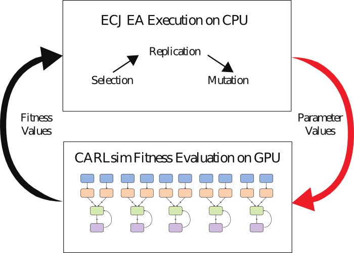
Source: Beyeler et al., 2015
7.2 Wrapping the Simulation
Let's begin by building our CARLsim model and fitness function. The full example is found in main_TuneFiringRates.cpp. You can use it as a template for implementing your own parameter-tuning experiments.
We'll do three things a little differently from the previous tutorials:
- we'll wrap our model in a CLI that accepts parameters on
stdin, - we'll use the
ParameterInstancesclass to handles parsing the input parameters and plug them into our model, and - after the model runs, we'll write a fitness value to
stdoutfor each parameter instance we received.
The Main Method
For the high-level entrypoint in main(), we'll start by including CARLsim and PTI.h. The latter cointains some high-level code that helps us standardize our parameter-tuning interface across projects (namely the Experiment and PTI classes).
Then we'll begin by loading a couple of CLI parameters. The verbosity parameter in particular will allow us to write CARLsim logs to stdout while we're debugging our model, but to keep them silent while tuning (so only fitness values are written to stdout). We're using a simple helper function hasOpt() for this (find it in the full source file):
Next, we'll instantiate our model. We'll write the implementation of TunefiringRatesExperiment class in a moment below:
To execute the model, we'll use the PTI class. This is a simple class that orchestrates the loading of parameters from an input stream (usually std::cin), uses them to execute your Experiment subclass, and collects the results to an output stream (std::cout).
The Experiment Class
Now, at the top of the same file, we'll implement the TuneFiringRatesExperiment class that our main() uses.
The layout of the SNN is as follows. We have a three groups of neurons, each configured to have NUM_NEURONS_PER_GROUP = 100 neurons:
- a group
poissonof excitatory, Poisson-spiking input neurons, - a group
excof excitatory regular-spiking (RS) neurons that receive this input, and - a group
inhof inhibitory fast-spiking (FS) izhikevich neurons that receive input from the excitatory RS neurons.
Additionally, inh is connected to the RS exh group, and exh is connected to itself recurrently. There are therefore 4 connection weight ranges to be tuned
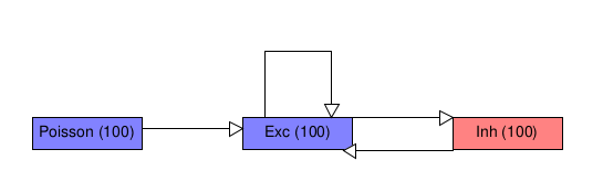
The goal of the our parameter-tuning problem is to make the RS exc group have an average firing rate of 10 Hz and make the FS inh group have an average firing rate of 20 Hz.
First we'll inhereit from the Experiment base class and define some constants used by our model. This makes it possible to pass our model into into a pti.runExperiment() call:
For our constructor, we'll just pull in two parameters to define whether we're using a CPU or GPU, and what level of logging to use.
Now we'll implement the run() method, which handles the simulation meat and acts as the fitness function for optimization.
Now we are going to build many neural networks at the same time within a single CARLsim instance—one for each of the parameter vectors in the ParameterInstances. Doing this allows us to evaluate several separate networks at once on a GPU.
We'll start by seting up SpikeMonitors and variables to track the neuron groups for each individual's network:
We'll also set up some more arrays to track the firing rates of each network, and the fitness values that we'll calculate from those firing rates:
Now we'll set up the actual groups for each network. This involves iterating through all of the ParameterInstances that we have been given, and using their values to set certain parameters of our network. These are the values that will be tuned to maximize our measure of fitness:
Now we need to pause and compile the networks before attaching the monitors:
Now we'll hop back into a for loop to add the monitors:
Now we can execute the networks:
After the simulation is complete, we can loop back through and compute fitness values for each network.
The fitness function can be whatever you need it to be to solve your problem: just compute a number and write it to the outputstream variable that is passed into the run() method.
In this tutorial, we compute fitness based on the difference between each group's mean firing rate and our target firing rate. We want our fitness function to define a maximization problem, where higher values are better (because ECJ expects to be given maximization problems). To achieve this, we sum the errors for each group and then take the reciprocal:
Lastly, we'll close our Experiment with some cleanup, since we didn't use smart pointers:
All done. Compiling main_TuneFiringRates.cpp yields a program TuneFiringRates that takes comma-delimited parameter vectors on std::cin and outputs fitness values.
7.3 The ECJ Parameter File
The other piece of the puzzle is the optimization algorithm. You can use anything you want to search the model's parameter space, but ECJ and CARLsim are specifically built to work together. ECJ offers a wide variety of evolutionary algorithms that can be used to tune complex, nonlinear parameter spaces.
We'll configure ECJ to optimize our model's parameter's with a simple evolutionary algorithm. To do so, we'll write a parameter file.
ECJ uses big, centralized parameter files to coordinate the interaction of a number of different algorithmic modules, traditionally ending with the extension .params (though they are in fact Java .properties files). In this example, we'll implement a (μ, λ)-style evolutionary algorithm (i.e., an algorithm that discards the parents at each generation) that evolves real-valued parameter vectors with Gaussian mutation of each real-valued gene, one-point crossover, and truncation selection. You can find the complete example in ecj_TuneFiringRates.params.
The ECJ manual is a great resource for undertstanding these parameters and how to configure them in more detail.
Boiler Plate
Create a new .params file and open it with an editor. We'll start by inheriting some boiler-plate parameters from a parent file at the top of our file:
The ecj_boiler_plate file contains quite a few standard parameter settings that we typically only alter in special circumstances—it defines things like the Java classes that manage the algorithm and population state.
Problem
Next, and most importantly, we want to tell ECJ to use an external binary program to compute fitness. This is done by configuring the problem parameter to point to the CommandProblem class. This is a special ECJ fitness function that writes parameters to a program's std::cin and reads fitness values back that your model writes to std::cout.
While we're at it we'll also define evalthreads, which controls how many instances of your model program will be run in parallel. In this tutorial we're relying on the internal parallelism of a single CARLsim instance to evaluate many individuals at once, so we'll leave ECJ's evalthreads set to 1.
Population
The next important group of parameters controls the population and the outline of how it evolves. Here we specify that we want a maximum number of 50 generations. The quit-on-run-complete parameter toggles whether or not evolution should stop early if a solution with the "ideal" fitness is found. We are tuning a noisy fitness function, however, which sometimes causes an individual to momentarily appear to have a high fitness by chance—and we don't want to stop early when that happens.
Now we'll tell ECJ to generate 20 individuals to populate the initial population (i.e. the very first generation, when individuals are generated randomly). It's sometimes a good idea to create many individuals in the first generation, because this gives us a chance to find a good starting point with random search, before we use evolution to refine it. After that, a (μ, λ) breeder takes over evolution, generating es.lamda.0 children and selecting es.mu.0 parents at each generation (the *.0 at the end of these parameter names refers to the settings for the "zeroeth subpopulation"; since we're using a single-population algorithm, this is the only subpopulation).
ECJ has several other breeding strategies available, including a (μ + λ) breeder (ec.es.MuPlusLambdaBreeder), which treats parents and offspring as a combined population (so parents have a chance of surviving multiple generations), and ec.simple.SimpleBreeder (which is like MuCommaLambdaBreeder, but is meant to work with other traditional selection methods, such as tournament selection).
Representation
Now we'll add several parameters to define how solutions are represented in the EA. The first three are pretty standard, specifying that we want to use floating-point vectors of numbers:
Now specify the numer of genes each individual should have, and the ranges within which they should be initialized. Our model has four parameters to tune, so we'll want four genes:
In this case we've configured all four parameters so that they share the same parameter range (0.0005, 0.5)—but each individual parameter can be given it's own range if need be (see the discussion of ECJ's "segments" mechanism in the ECJ manual).
Operators
The last algorithmic component we need to configure are the operators. These define how new individuals are created in each generation, and how parents are selected from the previous generation.
In ECJ, we add operators by stringing together "pipelines," each of which takes one or more source parameters. The following entries specify a pipeline that generates individuals via a mutation pipeline, taking its inputs from a crossover pipeline, which in turn receives individuals (in pairs) from an ESSelection operator. ESSelection performs truncation selection (i.e. it deterministically chooses the best individuals in the population). When the algorithm runs, ESSelection is applied first to the parent population, and mutation occurs last:
- Note
- The
ESSelectionoperator and theMuCommaLambdaBreeder(or, alternatively,MuCommaPlusBreeder) belong to ECJ's evolution strategies package,ecj.es, and are inteded to be used together. You cannot useESSelectionwithout one of these breeders, because they perform special bookeeping needed for elitist selection to work. Likewise, if you want to use other (less elitist) selection operators such asTournamentSelection, you may prefer to use ECJ's standardSimpleBreederinstead of these more complex breeders. See the ECJ manual for more information.
With the high-level pipeline in place, now we'll add parameters for the individual operators. The first set informs VectorMutationPipeline that we want to use additive Gaussian mutation, that we want mutation to be "bounded" (so that gene values cannot wander outside of their initial allowed range of 0.0005–0.5), and that we will always mutate every gene (probability 1.0) and use a mutation width (Gaussian standard deviation) of 0.5:
Next we'll define the crossover strategy, here choosing one-point crossover (which chooses one point to split individuals at when performing genetic recombination):
The selection operator ESSelection does not require any parameters, but if you use other operators (such as the popular TournamentSelection) they may have parameters of their own that you should also set.
Logging
By default, ECJ writes some information about the best individual found at each generation to stdout. If we want more information that this, we'll typically write it to a file. These two lines activate one of ECJ's statistics collection modules (SimpleStatistics) and point it to write to the file ./out.stat in the current directory.
Notice there is a $ in the output filename. This indicates that the output path an "execution-relative" path, i.e. it is relative to the working directory that the ECJ process was launched from (rather than relative to the parameter file we are writing). The different types of paths ECJ supporst are explained in the ECJ Manual.
Output
With our model compiled and our parameter file complete, we can tune the model by using the java command to run ECJ, passing in our parameter file to its -file argument:
The simulation should run to completion and output the best fitness each generation.
An out.stat file should also appear in the current working directory, since we configured the stat parameter to create it there. This will contains the best fitness for each generation along with the four parameter values associated with the individual. CARLsim users can then use these parameters for their tuned SNN models.
- Since
- v3.0
7.4 The LEAP Configuration File
Similar to using ECJ, we can also use LEAP to tune the network. A complete example can be found in leap_TuneFiringRates.params.
First we define the size of the population, the number of genes, and the maximum number of generations.
We then want to tell LEAP to evaluate an external problem, which launches the program that contains our network simulation.
We launch the evolutionary algorithm by calling the function generational_ea(...).
Here we specify that the solutions of the probelm are represented as real numbers, and the parameter range is (0.0005, 0.5). We then define the operator pipeline, which performs selection, mutation, and evaluation in sequence.
To launch the LEAP parameter tuning process, we can use the following command:
Input genomes and fitness information will be printed out like this:
References
Beyeler, M., Carlson, K. D., Chou, T. S., Dutt, N., Krichmar, J. L., CARLsim 3: A user-friendly and highly optimized library for the creation of neurobiologically detailed spiking neural networks. International Joint Confernece on Neural Networks (IJCNN), 2015.
Carlson, K. D., Nageswaran, J. M., Dutt, N., Krichmar, J. L., An efficient automated parameter tuning framework for spiking neural networks, Front. Neurosci., vol. 8, no. 10, 2014.
