|
CARLsim
3.1.3
CARLsim: a GPU-accelerated SNN simulator
|
|
CARLsim
3.1.3
CARLsim: a GPU-accelerated SNN simulator
|
In this tutorial, we introduce how to use some plasticity mechanisms in CARLsim. We will cover:
At the end of the tutorial, you will have:
This tutorial assumes you have covered:
The source code of this tutorial can be found in %%CARLSIM_ROOT_DIR%%/doc/source/tutorial/3_plasticity.
Spike timing-dependent plasticity (STDP) is a popular learning rule in spiking neural networks (SNNs). STDP was first found in neurons in 1997 and is still under intense study (Sjöström Gerstner (2010)). SNNs are a unique class of neural network (NN) models that capture the temporal dynamics (spike times) of the network. Because of this, they are ideally sutied to implement STDP. However, STDP can often undergo 'runaway potentiation' or 'runaway depotentiation' where the synaptic weights increase or decrease without bound, respectively. To avoid this, CARLsim users can utilize a model of homeostatic synaptic scaling implemented in CARLsim. The homeostatic synaptic scaling model (Carlson et al., 2014) is biologically plausible and works as follows. The average firing rate of each neuron is calculated over a time period on the scale of minutes to hours. This average firing rate is compared to a user-defined target firing rate and the difference between these firing rates is used to scale all synapses on that neuron up or down multiplicatively. For instance, if a neuron has an average firing rate of 10 Hz and a target firing rate of 20 Hz, it will scale up all postsynaptic weights on that neuron in an effort to attain the target firing rate.
In this tutorial, we will show users how to configure and enable both STDP and homeostasis in a simple model. This tutorial does not currently cover using short-term plasticity (STP). For more information on STP, please see: 5.1 Short-Term Plasticity (STP). The network we construct will have 100 Poisson input neurons connected to a single regular spiking (RS) output neuron. Every synaptic connection between the input neurons and the output neuron will be plastic and have both STDP and homeostasis enabled. Each input neuron will be assigned a different input firing rate in ascending order from 0.2 Hz to 20 Hz. The synaptic weights will be randomly initialized and the simulation will then run for 1000 seconds. The spike and synaptic weight data will be visualized using the MATLAB OAT scripts provided in the: %%CARLSIM_ROOT_DIR%%/doc/source/tutorial/3_plasticity/scripts. Users will see that homeostasis can successfully stabilize STDP by visualizing the weights before and after the 1000 seconds of simulation.
As always, the first step in setting up a CARLsim program is to include the libCARLsim library. We also include the vector library because we will be using the vector data structure.
We first construct a simple SNN that has 100 Poisson input neurons (group ID = gPoiss) all connected to a single regular spiking (RS) Izhikevich output neuron (group ID = gExc) as shown below. Notice we passed the GPU_MODE argument in our CARLsim constructor call. This means our simulation will take place on the GPU. Also notice that the last argument for CARLsim::createSpikeGeneratorGroup is EXCITATORY_POISSON and not EXCITATORY_NEURON. The setNeuronParameters call assigns the RS spiking neuron parameter values to all neurons in the gExc group.
We next connect neurons from the gPoiss group to neurons (just one for now) in the gExc group with full connectivity with a minimum weight value of 0.0, an initial value of 1.0f/100, and a maximum value of 20.0f/100. The connection probability is given as 1.0f, a delay of 1 is used for all synapses, and no receptive fields are specified (-1). Finally, the keyword 'SYN_PLASTIC' is used instead of 'SYN_FIXED' to enable plasticity for this connection. This is required. Also, the simulation is set to use conductances with default parameter values with the CARLsim::setConductances call.
A PoissonRate object is then created to use as an input to a SpikeGenerator group. It is the same size of as the SpikeGenerator group and is allocated on the GPU for efficiency.
Next, enable excitatory STDP (E-STDP) with a call to CARLsim::setESTDP pass the postsynaptic group you want to enable it for and 'true' to enable it. Additionally, the 'STANDARD' keyword indicates that there will not be a neuromodulatory influence at this synapse. Finally, the STDP curve type is specified by passing the stdpCurve_t data type with the desired STDP parameters. alpha_LTP(alpha_LTD) represents the magnitude of the increase(decrease) in synaptic weight while tau_LTP(tau_LTD) represents the time constant, which defines the width of the LTP(LTD) curve with respect to time. Notice that alpha_LTD is passed as being negative. The alpha_ltp and alpha_ltd parameters are allowed to be positive or negative depending on the user's preference. This allows users to build the many different type of EXP_CURVE type STDP curves found in 5.2 Spike-Timing Dependent Plasticity (STDP), Fig. 2(a-d) and 2(f-i). The tau_LTP/tau_LTD parameters, however, cannot be negative as they are time constants.
It should be noted that the function call CARLsim::setSTDP could have replaced the CARLsim::setESTDP function call, as it is a wrapper for this function call. However, the CARLsim::setESTDP is unambiguous and is therefore the preferred method.
Homeostatic synaptic scaling parameters are next defined. The homeostatic scaling factor (homeoScale) defines how large the effect of homeostasis will have the synaptic weight change. The synaptic weight change is composed of two terms, the homeostatic term and the STDP term. Each term has a scaling factor associated with it. The STDP scaling term has a value of 1. Therefore, to give the homeostatic term a larger influence than the STDP term, increase the homeostatic scaling factor to a value greater than 1. The homeostatic time constant (avgTimeScale) term defines the length of time over which the average firing rate of neurons in this group are calculated during the homeostasis calculation. Finally the target firing rate (targetFiringRate) term defines the firing rate the neurons in the group will attempt to attain.
To enable homeostasis, the CARLsim::setHomeostasis function is called with the postsynaptic group as the first argument, a boolean flag that enables/disables homeostasis as a the second argument, the homeostatic synaptic scaling constant as the third argument, and the homeostatic time constant as the fourth argument. The CARLsim::setHomeostasis function can be called with just the first two arguments, in which case the default values of homeoScale = 0.1 and avgTimeScale = 10 will be used. When homeostasis is enabled, users must also define the target firing rate neurons in the group. This is done with a call to CARLsim::setHomeoBaseFiringRate, where the postsynaptic group, value of the targetFiringRate, and the standard deviation of the targetFiringRate are specified by the user. Please note that the target firing rate is calculated once at the beginning of the simulation and remains the same throughout the simulation.
Chapter 5: Synaptic Plasticity
During the SETUP state of CARLsim, CARLsim::setupNetwork is called. Two SpikeMonitor pointers are declared and assigned SpikeMonitor objects created with the CARLsim::setSpikeMonitor function call. The first argument to these functions is the group for which the spike data will be recorded while the second argument is the filename of the spike data files. The argument of "DEFAULT" denotes that the default filename conventions will be used, namely: "results/spk_{group name}.dat". We also create a ConnectionMonitor to record the synaptic weights for the connection between the input group and the output group. The CARLsim::setConnectionMonitor function is used, with the first argument being the presynaptic group, the second argument being the postsynaptic group, and the third argument the name of the filename. We use 'DEFAULT' which assigns the string: "results/conn_{pre-group name}_{post-group name}.dat" to the filename. Finally, we disable the automatic output of ConnectionMonitor by using the function call ConnectionMonitor::setUpdateTimeIntervalSec with an argument of -1. We will output the weight values manually, later in the simulation.
During the RUN state, we set the firing rates of each of the nPois (100) neurons. We assign the first input neuron an average firing rate of 0.2 Hz, the second input neuron an average firing rate of 0.4 Hz, and so on. This gives our 100th input neuron an average firing rate of 20 Hz. We can now observe the weight change at each input/output synapse as a function of the average firing rate of the input neurons each having Poisson firing statistics.
We first generate a vector that contains the average firing rate for each Poisson neuron with the following code:
The vector is then passed to the PoissRate object and the poissRate is assigned to the gPois group with the following two calls. Additionally, we define the runTimeSec and runTimeMs variables explicitly here. This is common practice as there are often multiple calls to runNetwork with different run times for each call.
Finally, we take a snapshot of the weights between the input and output groups before we run the simulation, run the simulation, and then take a snapshot of the weights after the simulation has been run. This is shown in the code below:
In Linux, after navigating to %CARLSIM_ROOT_DIR%%/doc/source/tutorial/3_plasticity, the network can be compiled and run with the following commands:
In Windows, the .vcxproj file is already added to the CARLsim.sln solution file. Thus the project can be built simply by opening the solution file in Visual Studio, by right-clicking the project directory and choosing "Build project".
Some of the CARLsim output is shown below:
Notice that the simulator notifies you that E-STDP has been enabled for output(1). The (1) denotes the group ID. It also notifies you that homeostasis is enabled for the output group and details the exact parameter values being used.
During the network setup, the simulator lists the parameter values for E-STDP. Here we see that 'STANDARD' is selected as well. Notice that we are notified that two SpikeMonitors have been set, one for 0 and one for group 1. Finally, we are notified that a ConnectionMonitor has been set for the conncection between group 0 and group 1. The '...' denotes excluded output.
CARLsim also outputs information about the synaptic weight strengths and their recent changes in synaptic weight. Below we see presynaptic neuron id and postsynaptic neuron id in brackets, indicating the specific synapse. For example [ 0, 0] indicates the synaptic connection from presynaptic neuron 0 to postsynaptic neuron 0. Here, you can see all synaptic connections have the same postsynaptic neuron id (0), meaning these are connections from many different presynaptic neurons to a single postsynaptic neuron. Next, is the value of the synaptic weight with the change in the last second in parenthesis. For example: 0.0016 (+0.0004) indicates that the weight has a value of 0.0016 and has increased 0.0004 in the past 1 second.
Finally, we see the number of neurons involved in the total simulation (numNeurons = 101), the total number of synapses (numSynapses = 100), and the overall average firing rate: (Overall = 10.368 Hz).
In order to plot network activity and observe weight changes in the network, we will make use of the MATLAB Offline Analysis Toolbox (OAT) (see Chapter 9: MATLAB Offline Analysis Toolbox (OAT)). The CARLsim simulation will output spike and synaptic weight data files to the results directory. To run, the network visualization scripts, simply open MATLAB, change the current directory to the "scripts/" directory and run:
The plasticityOAT.m script looks like this:
After adding the location of the OAT source code to the MATLAB path, a SpikeReader is opened on the spike data file: "../results/spk_output.dat" which was created during the CARLsim simulation because we created a SpikeMonitor.
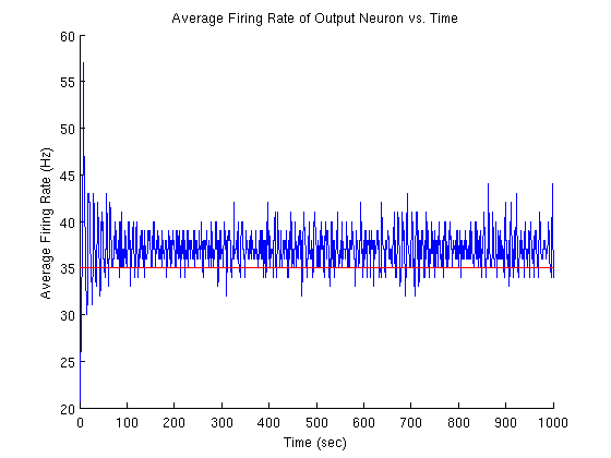
Calling the readSpikes method with an argument of '1000' creates 1000 ms wide bins in which it places the total number of spikes for that time period (1000 ms). The user can then easily create a plot or histogram with the data. Below Fig. 1 shows the target firing rate and actual average firing rate of the output neuron.
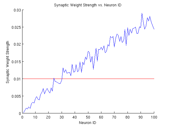
To visualize the weights, we next open a ConnectionReader on the file "../results/conn_input_output.dat" which was created during the CARLsim simulation because we created a ConnectionMonitor. We use the readWeights method to return a matrix that contains the time stamps of when each synaptic weight snapshot was created. The synaptic weight values are output to the allWeights matrix. See the code comments for more information. Finally, we plot the initial weight values in red and the final weight values in blue as shown in Fig. 2.
 1.8.11
