We will first use the VisualStimulus toolbox to generate a drifting sinusoidal grating. Then we will use the MotionEnergy library to parse the stimulus and generate direction-selective responses akin to those of neurons in the primary visual cortex (V1). These responses will then be assigned to a spike generator group, which we term V1. A second group, termed middle temporal area (MT) neurons, will then sum over V1 responses using a Gaussian kernel in space (x and y), but not direction (z).

At the end of the tutorial, you will know how to:

generate a drifting sinusoidal grating using the VisualStimulusToolbox
parse a stimulus using the MotionEnergy library
assign MotionEnergy output to SpikeGenerator groups
use the Grid3D and RadiusRF structs for 2D and 3D transforms
create Gaussian connections for neurons arranged on a 2D/3D grid

The source code of this tutorial can be found in %%CARLSIM_ROOT_DIR%%/doc/source/tutorial/5_motion_energy.

5.1 The MotionEnergy Library

The MotionEnergy library provides a CUDA implementation of Simoncelli and Heeger's Motion Energy model (Simoncelli & Heeger, 1998). The code itself is based on Beyeler et al. (2014), and comes with both a Python and a C/C++ interface.

In this tutorial, we will make use of the C/C++ interface. For this, we first have to install the library.

5.1.1 Installing the Library

If you followed the CARLsim installation instructions outlined in Chapter 1: Getting Started, you already have the code in external/MotionEnergy.

However, if your external/MotionEnergy directory appears to be empty (e.g., because you forgot the –recursive flag when you cloned CARLsim), you have to initialize the submodule yourself. Simply navigate to the CARLsim root directory and run the following:

$ git submodule update --init --recursive

Then navigate to the library directory to compile and install the code.

$ cd external/MotionEnergy/cppME
$ make
$ sudo make install

This will install the library to /opt/CARL/ME. If you wish to install it in a different library, you can export an environment variable ME_LIB_DIR prior to compiling:

$ cd external/MotionEnergy/cppME
$ export ME_LIB_DIR=/path/to/your/preferred/dir
$ make install

5.1.2 First Steps

You can verify the installation by running the example project:

$ cd external/MotionEnergy/cppME/projects/hello_world
$ make
$ ./hello_world

5.2 Stimuli

In order to create a visual stimulus depicting a drifting sinusoidal grating, we will make use of the VisualStimulusToolbox.

If this is your first time using the toolbox, have a look at 4.1 VisualStimulusToolbox to make sure it is correctly installed.

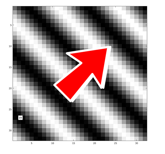
The easiest way to create the stimulus is to run the script script/createGratingVideo.m. What it does is, it creates a 32x32 pixel grating using GratingStim:

>> initOAT
>> grating = GratingStim([32 32])
grating = 
  GratingStim with properties:
                  width: 32
                 height: 32
               channels: 1
                 length: 0
                   stim: []
    supportedNoiseTypes: {'gaussian'  'localvar'  'poisson'  'salt & pepper'  'speckle'}

We can then add frames to empty stimulus by specifying the number of frames and the direction of motion in degrees, where 0 stands for rightward motion, 90 deg is upward, 180 deg is leftward, and 270 deg is downward. Here we want to sample the spectrum in 45 deg increments, and add 10 frames each:

>> for dir=(0:7)*45
..    grating.add(10, dir)
.. end

This should have added 80 frames to the object.

Note: Check out help GratingStim.add to find out how to change the spatial frequency of the grating, as well as other parameters.

You can always have a look at what you created by using plot:

>> grating.plot

Example frame of the drifting sinusoidal grating.

Last thing to do is save the stimulus to file:

>> grating.save('../input/grating.dat')

Note: Gratings aren't the only stimulus supported by the toolbox. You can also create plaids using PlaidStim, random dot fields using DotStim, drifting bars using BarStim, a combination of all of the above—or you can simply load a video using MovieStim. Check out the documentation for more!

5.3 Network

Now it is time to set up the CARLsim network.

5.3.1 Importing the Stimulus

If you have worked through the previous tutorial, you should already know how to do this. The idea is to assign every pixel in the stimulus to a neuron in the spiking network. In order to preserve spatial relationships, we arrange all neurons on a grid that matches the image dimensions.

The stimulus is imported simply by:

VisualStimulus stim("input/grating.dat");

5.3.2 Assigning Image Pixels to Neurons

We can create a Grid3D struct from the stim dimensions. We want to create a population of V1 neurons that is selective for eight directions of motion. For this to work, we therefore need eight neurons per pixel location (each selective for a different direction of motion). We can simply assign motion direction to the third dimension of the grid struct. Hence the right Grid3D dimensions for V1 are:

int numDir = 8;

Grid3D gridV1(stim.getWidth(), stim.getHeight(), numDir);

We also want a grid for a population of MT neurons. We could use the same grid as for V1, but since there are more neurons in V1 than there are in MT, let's downscale the grid a bit:

Grid3D gridMT(stim.getWidth()/2, stim.getHeight()/2, numDir);

So all we need to do is create groups with the above grids:

// ---------------- CONFIG STATE -------------------
bool onGPU = true;
CARLsim sim("me", onGPU?GPU_MODE:CPU_MODE, USER);
int gV1=sim.createSpikeGeneratorGroup("V1", gridV1, EXCITATORY_NEURON);
int gMT=sim.createGroup("MT", gridMT, EXCITATORY_NEURON);
sim.setNeuronParameters(gMT, 0.02f, 0.2f, -65.0f, 8.0f);

We also want V1 to be input to MT. MT neurons should sum over V1 neurons using a Gaussian kernel in x and y (let's say a kernel the size of 7x7 pixels), but they should not sum over z (which is the direction of motion). In this way, MT neurons will preserve the direction selectivity of their V1 inputs. Hence the correct RadiusRF struct has size 7x7x0:

sim.connect(gV1, gMT, "gaussian", RangeWeight(0.02), 1.0f, RangeDelay(1), RadiusRF(7,7,0));

5.3.3 Setting up the MotionEnergy object

The MotionEnergy object is initialized with the size of the stimulus we imported above:

MotionEnergy me(stim.getWidth(), stim.getHeight(), stim.getChannels());

Its job is then to parse the stimulus frame-by-frame, and convert it to a float array of filter activation values. We will have exactly one filter value per neuron in the group, so it's possible to convert this activation value into spikes.

For this to work, we have to choose a frame duration: This means that every frame in the video is worth some number of milliseconds of simulation time, let's say 50 ms:

int frameDurMs = 50;

During this time, every neuron in the group will fire spikes according to a Poisson process (using the PoissonRate object), the mean rate of which has yet to be determined. This process will get clearer in a second, but for now let's just initialize the PoissonRate container and assign it to the V1 group:

PoissonRate rateV1(gridV1.N, onGPU);

sim.setSpikeRate(gV1, &rateV1);

5.3.4 Setting up the Network

After all this, don't forget to call CARLsim::setupNetwork and set a bunch of monitors:

sim.setConductances(true);
// ---------------- SETUP STATE -------------------
sim.setupNetwork();
sim.setSpikeMonitor(gV1, "DEFAULT");
sim.setSpikeMonitor(gMT, "DEFAULT");

Then we are ready to run the network.

5.3.5 Running the Network

This is where the magic happens. We will read a frame of the stimulus movie using VisualStimulus, pass the frame to the MotionEnergy object, and assign the output to the PoissonRate object of the V1 group. Bam!

First, we will parse the stimulus frame-by-frame, so we'll wrap all the action in a for loop:

// ---------------- RUN STATE -------------------
for (int i=0; i<stim.getLength(); i++) {
    // ...
    sim.runNetwork(frameDurMs/1000, frameDurMs%1000);
}

Two commands remain.

The first is how to read the next frame of the stimulus. This logic is all contained within VisualStimulus, so all you need to do is simply call the readFrameChar repeatedly to get an array of all grayscale values in an unsigned char* frame array that we initialized above:

frame = stim.readFrameChar();

This will automatically access the next frame in the queue.

Then we pass the frame to the MotionEnergy object. This object has methods that expose different intermediate steps of the Motion Energy model, such as the V1 linear filter response, the normalization step, and the V1 complex cell response. It is the latter that we want here:

me.calcV1complex(frame, onGPU?rateV1.getRatePtrGPU():rateV1.getRatePtrCPU(),

speed, onGPU);

This method takes a frame, processes it, and returns an array of filter values that gets written to the rateV1 container. Now, because all computations are performed on the GPU, it would be silly to copy the result from the GPU to the CPU, only to find out that the PoissonRate object also lives on the GPU—so we have to copy all data back. Instead, we want to pass the right pointer (rateV1.getRatePtrGPU() if the PoissonRate object was allocated on the GPU), and indicate that this is a pointer to device memory (using onGPU set to true).

After putting it all together, the run state code should look like this:

// ---------------- RUN STATE -------------------
for (int i=0; i<stim.getLength(); i++) {
  frame = stim.readFrameChar();
  me.calcV1complex(frame, onGPU?rateV1.getRatePtrGPU():rateV1.getRatePtrCPU(),
    speed, onGPU);
  sim.runNetwork(frameDurMs/1000, frameDurMs%1000);
}

And that's it!

5.3.6 Visualizing the Output

You can compile and run the above network as follows:

$ make motion_energy

$ ./motion_energy

The result can then be analyzed using the OAT. Visualizing network activity is easiest with the NetworkMonitor. Go back to the scripts folder in MATLAB, and run:

>> demoOAT

This script will first plot all network activity as heat maps:

Network activity as heat maps

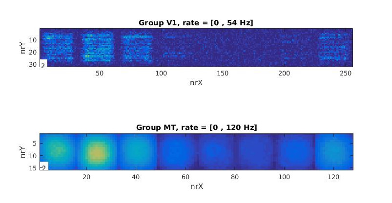
Here you can see group activity for V1 and MT over time. You can see hotspots of activity, which tends to run over the image from left to rigth as time moves on. The 8 "blobs" or subpopulations you see correspond to the 8 subpopulations of neurons we created above. Within these 8 subpopulations, we have all pixels of a stimulus frame represented, each pixel location encoded by a neuron. Thus the 8 subpopulations you see correspond to a 32x32 slice through the 32x32x8 grid of neurons.

As the drifting direction of the grating changes, so do the hotspots of activity. This is easiest to visualize using a flow field: Since we have 8 neurons coding for 8 different directions at each pixel location, we can use population vector decoding to find the net vector of motion that these 8 neurons encode. This is the second plot produced by the script:

Network activity as a flow field

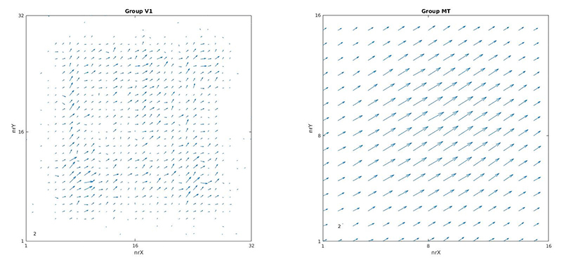
This should make things much clearer: As time moves on, the direction of motion judgment of the neurons changes as well. You can also see that V1 activity tends to be noisier, whereas the Gaussian smoothing performed by the MT population makes the motion appear much more coherent.

Note: In these plots, the angle of the vectors stands for direction of motion, and the length of the vectors stands for confidence in direction judgment, not speed as is common in optic flow fields.

Table of Contents