Table of Contents
2.1 General Workflow
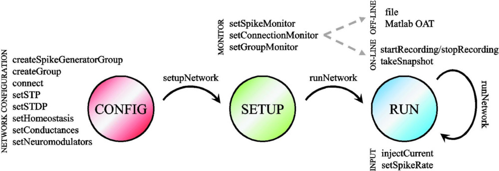
The workflow of a typical CARLsim 5 simulation is organized into three distinct, consecutive states (see figure below): the configuration state, the set up state, and the run state.
User functions in the C++ API are grouped according to these stages, which streamline the process and prevent race conditions. State transitions are handled by special user functions such as CARLsim::setupNetwork and CARLsim::runNetwork.
The first step in using CARLsim 5 (libCARLsim) imports the library and instantiates the main simulation object:
This prepares the simulation for execution in either CPU_MODE or GPU_MODE, and specifies the verbosity of the status reporting mechanism (USER indicating the default logger mode that will print info and error messages to console and save debug messages in a text file). Other logger modes are available that print only error messages (SHOWTIME), suppress console output alltogether (SILENT), or allow to set custom file pointers for each message type (CUSTOM).
The ability to run a network either on standard x86 CPUs (CPU_MODE) or off-the-shelf NVIDIA GPUs (GPU_MODE) allow the user to exploit the advantages of both architectures. Whereas the CPU is more efficient for relatively small networks, the GPU is most advantageous fo rnetwork sizes of 10,000 neurons and up. In this regime, GPU mode should significantly outperform CPU mode (with roughly a factor of 20). On the other hand, CPU mode allows for execution of extremely large networks that would not fit within the GPU's memory.
In addition, the user may want to specify on which CUDA device to run the simulation. For this, the CARLsim constructor allows specification of a "device index" (ithGPU, which can be used in multi-GPU systems to specify on which CUDA device to establish context. For example, in order to run a network on the third GPU in the system (ithGPU=2, 0-indexed) and use random seed 42, the constructor should be called as follows:
From then on, the simulation is in CONFIG_STATE, allowing the properties of the neural network to be specified.
2.1.1 The CONFIG State
Similar to PyNN and many other simulation environments, CARLsim uses groups of neurons (see Chapter 3: Neurons, Synapses, and Groups) and connections (see Chapter 4: Connections) as an abstraction to aid defining synaptic connectivity. Different groups of neurons can be created from a one-dimensional array to a three-dimensional grid (see 3.3.2 Topography) via CARLsim::createSpikeGeneratorGroup or CARLsim::createGroup, and connections can be specified depending on the relative placement of neurons via CARLsim::connect. This allows for the creation of networks with complex spatial structure.
The present release allows users to choose from a number of synaptic plasticity mechanisms (see Chapter 5: Synaptic Plasticity). These include standard equations for STP (see 5.1 Short-Term Plasticity (STP)), various forms of nearest-neighbor STDP (see 5.2 Spike-Timing Dependent Plasticity (STDP)), and homeostatic synaptic plasticity in the form of synaptic scaling (see 5.3 Homeostasis).
For a selective list of available function calls in CONFIG_STATE, please refer to the left-hand side of the above figure.
2.1.2 The SETUP State
Once the spiking network has been specified, the function CARLsim::setupNetwork optimizes the network state for the chosen back-end (CPU or GPU) and moves the simulation into SETUP_STATE.
In this state, a number of monitors (see Chapter 7: Monitoring) can be set up to record variables of interest (e.g., spikes, weights, state variables) in binary files for off-line analysis (see Chapter 9: MATLAB Offline Analysis Toolbox (OAT)). New in CARLsim 5 is a means to make these data available at run-time (without the computational overhead of writing data to disk), which can be queried for data in the RUN_STATE.
For example, Spike Monitors can be used to record output spikes for different neuronal groups (see 7.1 Spike Monitor) either to a spike file (binary) or to a SpikeMonitor object. The former is useful for off-line analysis of activity (e.g., using Chapter 9: MATLAB Offline Analysis Toolbox (OAT)). The latter is useful to calculate different spike metrics and statistics on-line, such as mean firing rate and standard deviation, or the number of neurons whose firing rate lies in a certain interval.
Similar monitors exist to record weights (see 7.2 Connection Monitor). More monitors will be added in the future.
2.1.3 The RUN State
The first call to CARLsim::runNetwork will take the simulation into RUN_STATE. The simulation can be repeatedly run (or "stepped") for an arbitrary number of sec*1000 + msec milliseconds:
Input can be generated via current injection (see 6.2 Generating Current) or spike injection (see 6.1 Generating Spikes). We also provide plug-in code to create Poisson spike trains from animated visual stimuli such as sinusoidal gratings, plaids, and random dot fiels via the VisualStimulus MATLAB toolbox (see 6.3 Visual Stimulus Toolbox).
Once a network has reached CONFIG_STATE or RUN_STATE, the network state can be stored in a file for later processing or for restoring a specific network (see Chapter 8: Saving and Loading). The network state consists of all the synaptic connections, weights, delays, and whether the connections are plastic or fixed. Furthermore, the network can be stored after synaptic learning has occurred in order to externally analyze the learned synaptic patterns (for example, via a MATLAB ConnectionMonitor; see ch9s4_connection_monitor).
As more complex biological features are integrated into spiking network models, it becomes increasingly important to provide users with a method of tuning the large number of open parameters. To this end, CARLsim 5 provides a paramer tuning interface that uses evolutionary algorithms to optimize a generic fitness function (see Chapter 10: ECJ). A more modest approach is to use the SimpleWeightTuner utility that changes weights on-the-fly such that a certain group fires at a predefined target firing rate (see ch12s3_online_weight_tuning).
As mentioned before, once a network has been run, its activity and structure can be visualized using an Offline Analysis Toolbox (OAT) written in MATLAB (see Chapter 9: MATLAB Offline Analysis Toolbox (OAT)). In addition, the OAT provides means to access the saved data programmatically, and to store generated sequences of plots as an AVI file.
- See also
- Tutorial 1: Basic Concepts