Table of Contents
- See also
- Chapter 1: Getting Started
- Chapter 2: Basic Concepts
- Chapter 3: Neurons, Synapses, and Groups
- Chapter 4: Connections
- Chapter 9: MATLAB Offline Analysis Toolbox (OAT)
In this tutorial we will implement one of the smallest functional CARLsim simulations, consisting of a Poisson spike generator connected to an Izhikevich neuron with a single fixed (non-plastic) synapse. We will run the network for a total of ten seconds, during which time the firing activity of the Izhikevich neuron will be recorded and dumped to file. We will then visualize the firing activity using a GroupMonitor from the MATLAB Offline Analysis Toolbox (OAT).
At the end of the tutorial, you will know how to:
- import the CARLsim library and instantiate the simulation object
- create groups of neurons
- specify the network structure by connecting neurons
- run a network on the CPU and GPU
- use a GroupMonitor to visualize neuronal activity (OAT)
This tutorial assumes you know:
- the very basics of C/C++
- the Izhikevich neuron model
- how to install CARLsim
The source code of this tutorial can be found in %%CARLSIM_ROOT_DIR%%/doc/source/tutorial/1_basic_concepts.
1.1 A Simple CARLsim program
The smallest functional CARLsim network contains just two neurons, connected with a single synapse.
After successful installation, the first step in setting up a CARLsim program is to include the libCARLsim library and to instantiate the main simulation object:
This prepares the simulation for execution in either CPU_MODE or GPU_MODE, and specifies the verbosity of the status reporting mechanism, where USER indicates the default logger mode that will print info and error messages to console and save debug messages in a text file. By default, this file is called "carlsim.log" and can be found in the "results/" subdirectory.
Running a simulation on the GPU is as easy as replacing CPU_MODE with GPU_MODE in the above code. No other adjustments are necessary. However, it is possible to pass an additional input argument ithGPU to specify the device index (on which GPU to run in a multi-GPU system).
1.1.1 CONFIG State
From then on, the simulation is in CONFIG_STATE, allowing the properties of the neural network to be specified. In this tutorial, we consider a network with two neuronal groups, each of which contains a single neuron.
A SpikeGenerator group is created by specifying a name for the group ("input"), the number of neurons in the group (just one), and a type (EXCITATORY_NEURON):
To refer to this group in later method calls, a group ID is returned (gIn). A SpikeGenerator is different from an Izhikevich neuron in that it does not provide a differential equation of its membrane potential; instead it only contains a list of spike times.
Similarly, a group of Izhikevich spiking neurons can be created by specifying a name for the group ("output"), the number of neurons in the group (again just one), and a type (EXCITATORY_NEURON). However, in contrast to the SpikeGenerator group, we also need to specify the Izhikevich parameters a, b, c, and d. These two things can be achieved with the following code snippet:
where we use the ID gOut to refer to the group, and set a=0.02f, b=0.2f, c=-65.0f, and d=8.0f (regular spiking).
Then the synaptic connections can be specified. The two groups are connected with the "one-to-one" primitive type of CARLsim::connect that connects neuron i in the pre-synaptic group to neuron i in the post-synaptic group (both groups must have the same number of neurons):
where we initialize and fixate the weight magnitude at 0.05f and set the connection probability to 1.0f (100%). We use default values for the other input arguments (1 ms axonal delay, no particular spatial receptive field, and a non-plastic synapse type, SYN_FIXED).
As a side note: Since there is only one neuron in each group, "one-to-one" connectivity would have the same effect as "full" connectivity or "random" connectivity with 100% connection probability.
Finally, we enable synaptic conductances so that the network is run in COBA mode (see 3.2.2 COBA):
1.1.2 SETUP State
Once the spiking network has been specified, the function CARLsim::setupNetwork optimizes the network state for the chosen back-end (CPU or GPU) and moves the simulation into SETUP_STATE:
In this state, we specify a SpikeMonitor object to record network activity to a "DEFAULT" binary file (see Chapter 7: Monitoring):
This will dump all spikes of group gOut (in AER format) to a binary with default file name "results/spk_output.dat", where "output" is the name that was assigned to the group gOut in the call to CARLsim::createGroup above.
1.1.3 RUN State
The first call to CARLsim::runNetwork will take the simulation into RUN_STATE.
We will run a simulation for a total of ten seconds, during which the firing activity of group gOut will be recorded by using the SpikeMonitor set above.
At the beginning of the simulation, the spike generator group gIn will generate Poisson spike trains with 10Hz mean firing rate, but this number will be gradually increased every second until it reaches 100Hz.
1.2 Network Output
After navigating to %CARLSIM_ROOT_DIR%%/doc/source/tutorial/1_basic_concepts, the network can be compiled and run with the following commands (on Unix):
On Windows, the .vcxproj file is already added to the CARLsim.sln solution file. Thus the project can be built simply by opening the solution file in Visual Studio, by right-clicking the project directory and choosing "Build project".
Some of the CARLsim output is shown below:
The SpikeMonitor object produced one line of output at the end of every simulated second via implicitly calling SpikeMonitor::print. We observe a gradual increase of the output firing rate, which coincides with the gradual increase of input stimulation. Shown in parentheses on these lines are the mean firing rate of all neurons in the group (although there is only one neuron) and the standard deviation.
At the end of the simulation a summary is printed, informing about the number of neurons and synapses created. The network was simulated for 10 seconds, yet its execution took only 0.01 seconds of wall-clock time, which means the network was run 1000 times faster than real-time.
1.3. Visualizing Network Activity
In order to plot network activity and observe weight changes in the network, we will make use of the MATLAB Offline Analysis Toolbox (OAT) (see Chapter 9: MATLAB Offline Analysis Toolbox (OAT)).
1.3.1 Group Monitor
The Tutorial subdirectory "scripts/" provides a MATLAB script "scripts/demoOAT.m" to demonstrate the usage of the OAT. The script looks like this:
After adding the location of the OAT source code to the MATLAB path, a GroupMonitor is opened on the group with name "output" whose spike file resides in "../results". This group is the same as the one assigned name "output" and ID gOut in the code above (see 1.1.1 CONFIG State), and the reason a spike file "results/spk_output.dat" exists is that a SpikeMonitor was called on the group with "DEFAULT" file name (see 1.1.2 SETUP State).
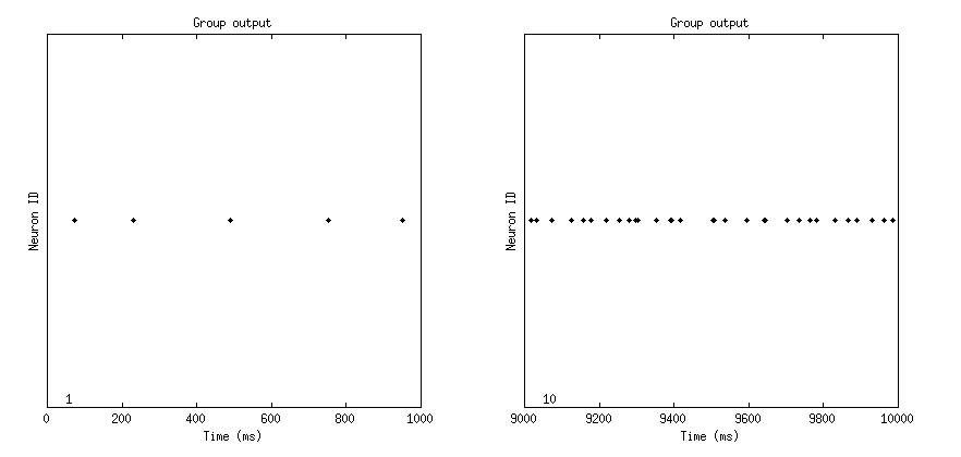
Calling the plot method will then visualize group activity using default settings and a plot type that depends on the spatial structure of the neuron group. Since the network does not have any particular spatial structure, the default plot type is a raster plot, shown in frames of 1000ms, as seen in Fig. 1 below.
1.3.2 Input-Output Curve (FF Curve)
Alternatively, it is also possible to directly access the raw spike data by means of a SpikeReader. The Tutorial subdirectory "scripts/" provides a MATLAB script "scripts/ffcurve.m" to demonstrate the use of a SpikeReader. Its contents read as follows:
After adding the location of the OAT source code to the MATLAB path, a SpikeReader is opened on the exact path to the spike file, "../results/spk_output.dat". The SpikeReader allows to manipulate raw spike data directly, but it will not know how to plot things (as opposed to the OAT GroupMonitor), and it will not be aware of other groups in the network (as opposed to the OAT NetworkMonitor).
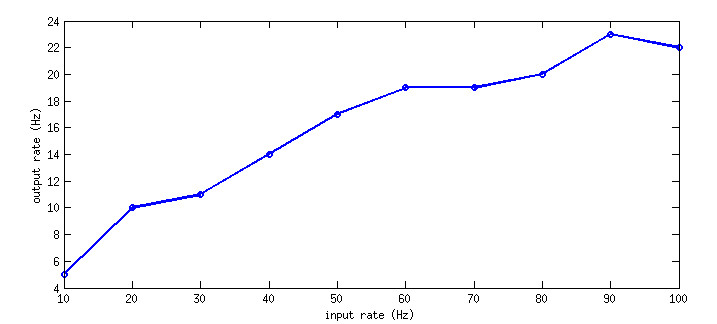
Calling the readSpikes method will then parse the spike data and return the number of spikes binned into 1000ms bins. Since there is only a single neuron in the group, the returned data will be in 1D (vector) format, where the first element in the vector will contain the number of spikes the neuron emitted during the first 1000ms of the simulation (from t=0 until t=999ms).
All that's left to do is then to plot these numbers (y-axis) vs. the corresponding input firing rate (x-axis). The latter is specified as a vector 10:10:100 containing the input firing rates in Hz. The result is shown in Fig. 2 below.
Alternatively, it would have been possible to emulate the GroupMonitor plot from above (see 1.3.1 Group Monitor) by calling the readSpikes method with value -1 instead, which is code for returning spikes in AER format. Producing a raster plot would then have been as easy as:
For users of CARLsim 2.2, please note that the readSpikes method of SpikeReader is essentially the same as the no longer existing MATLAB script readSpikes.m (see 9.6 Migrating from CARLsim 2.2).